Three oil analysis techniques were applied to used oil samples from an engine that was run in a test cell. The three techniques were Automatic Wear Particle Shape Classification, Ferrography and Spectroscopy. The analytical results from the techniques were compared to determine their effectiveness in working individually, or in combination, to rapidly determine engine condition based on oil analysis.
This paper details and reviews analytical results from the three techniques over the 540 hours of engine operation. A total of 31 samples were taken from start to finish. All samples were analyzed with an atomic emission spectrometer and the analytical results for twenty-one elements were recorded. The same samples were analyzed with the LaserNet Fines-C Particle Shape Classifier in order to obtain particle distribution and particle shape classification information. Ferrograms were prepared for morphological analysis with an optical microscope from key oil samples during break-in, steady wear and towards the end of the engine test.
The summarized data shows good correlation among the three techniques. Each in itself was able to identify wear trends. However, from a practical standpoint, the data show that spectroscopy combined with automatic wear particle shape classification provides a rapid means to determine detailed engine condition, and can be used together as a screening tool before ferrographic analysis needs to be undertaken.
Introduction
The purpose of this study was to investigate the correlation of three analytical techniques in their ability to determining wear trends on used oil samples. An engine manufacturer provided a total of 31 used oil samples from a test cell for this purpose. The three instruments used to analyze the oil sample were a LaserNet Fines-C (LNF-C) Particle Shape Classifier and Particle Counter, a Spectroil M/C Oil Analysis Spectrometer, and a T2FM Ferrography Laboratory. A secondary objective of the test program was to evaluate the shape recognition features of the LNF-C and compare them to the more conventional morphological analysis technique of ferrography using the T2FM Ferrogram Maker and the optical microscope.
The LaserNet Fines-C is a bench-top automated oil debris analysis instrument, Figure 1. It uses laser imaging techniques and advanced image processing software to identify the type, rate of production, and severity of mechanical faults by measuring the size distribution, rate of progression, and shape features of wear debris in lubricating oils or hydraulic fluids. The LNF-C does not require any special sample preparation prior to analysis, nor consumables such as electrodes or gases.
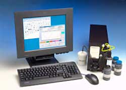
Figure 1. LaserNet Fines-C
Total analysis time for the oil samples in this report was approximately 2.5 minutes per sample. The Ferrography Laboratory, Figure 2, consists of the T2FM Ferrogram Maker and a bichromatic microscope. The ferrogram maker is used to separate magnetic and partially magnetic particles from the used oil sample onto a substrate so that an expert may view them through a bichromatic microscope to make his interpretation. Total sample preparation and analysis times varied from 15 minutes to up to 30 minutes per sample.
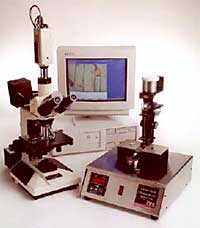
Figure 2. T2FM Ferrography Laboratory
The Spectroil M/C Oil Analysis Spectrometer is a bench-top atomic emission spectrometer based on the rotating disc electrode (RDE) technique, Figure 3. It provides simultaneous analysis of wear metals, contaminants and additives in lubricants and hydraulic fluids. The instrument used in these tests was capable of providing analytical results for 21 elements without any special sample preparation. Analysis times for the oil samples in this report was approximately 1 minute per sample.
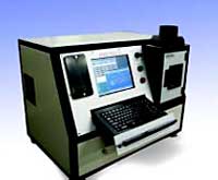
Figure 3. Spectroil M/C Oil Analysis Spectrometer
Procedure
A complete case history of all 31 engine samples were analyzed using the LNF-C and the Spectroil M/C. From the LNF-C results, specific samples from the set were chosen for a more in-depth morphological analysis using the T2FM Ferrogram Maker and the optical microscope. Since the samples were stored for several weeks, they were first thoroughly shaken using an automatic shaker in order to get any particles back into suspension. The samples were also shaken by hand for another thirty seconds prior to their analysis with each of the instruments. The samples were also placed in an external ultrasonic bath for 45 seconds to remove air bubbles prior to their analysis with the LNF-C.
Results
A tremendous amount of data was collected with the three instruments. Some of it was redundant, some was of no significance; however, the majority of the analytical results provided an excellent insight into the mechanical health of the engine in the test cell through the analysis of 31 samples over approximately 540 hours of operation. Figure 4 is a screen shot taken from the trending feature of the LNF-C. It shows the trend for the total number of particles for the 31 samples that were analyzed. The curve shows a “bath tub” shape that is typical of the wear cycle over the life of a particular machine. The wear stages are break-in followed by normal steady wear and then finally wear out to failure.
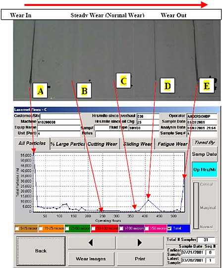
Figure 4. Different stages of the wear cycle as depicted by LNF-C and Ferrograms
Ferrograms were prepared from various oil samples at different wear stages of the test shown as A through E in Figure 4. The deposition of ferrous debris on the various ferrograms correlated very well with the quantitative results given by the LNF-C. The comparison between the two is shown in Figure 4 as photographs of the actual ferrograms compared against where they were taken along the trend as determined by the LNF-C.
Of the 21 elements that were analyzed with the Spectroil M/C oil analysis spectrometer, only five elements exhibited wear and trends; the remaining elements were either additives or present in insignificant concentrations. The analytical results for iron, aluminum, copper and silicon are shown in Figure 5. The superimposed letters are to depict the test cell hours at which ferrograms were also prepared.
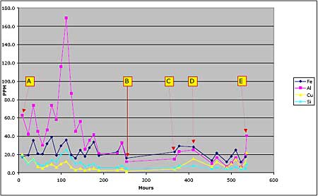
Figure 5. Spectrometric analysis trends
We do not know the type of test that was conducted on the test cell, but the oil was completely changed at least 15 times in the 540 hours of operation. It was never allowed to remain in the engine for more than 33 hours and was also changed every 10 hours between 450 and 500 hours of operation. The oil changes are evident in Figure 5 from the valleys (low concentration points) in the trends for each element.
The five stages of the test (numbered A through E) at which ferrograms were prepared and analyzed will be used to show correlation between the three analytical techniques.
Sample A – 8.8 Engine Hours - Break-in Wear
The LNF-C wear summary result during break-in is shown in Figure 6a. The total number of particles greater than 4 ìm detected and counted was 57,278/ml. The number of particles that were greater than 20 ìm are shown in the cutting, severe sliding, fatigue and non-metallic wear categories. The LNF-C image map of particle silhouettes for these particles is shown in Figure 6b. The majority of large particles as identified by LNF-C and quantified in the wear summary were severe sliding and fatigue particles. This fact was confirmed by ferrography through the digital photographs as shown in Figure 6c. The first particle shown in Figure 6c is an excellent example of severe sliding wear and clearly shows the characteristic sliding marks (parallel lines) across the surface. Spectrometric oil analysis of sample A, as shown in Figure 5, shows a higher level of wear metals for aluminum, copper and silicon. One would not expect extremely high concentrations of wear particles during break-in, because these particles tend to be larger than the 10 ìm particle size detection capability of RDE spectroscopy. This fact is confirmed in the particle image map and ferrograms.
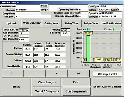
Figure 6a. LNF-C Wear Summary Screen, 8.8 Hrs
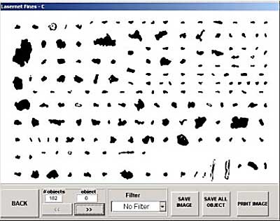
Figure 6b. LNF-C Particle Image Map
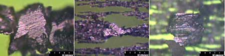
Figure 6c. Photographs of ferrograms showing severe sliding wear during break-in
Sample B - 254 Engine Hours- Normal Running (Mild Wear)
The LNF-C wear summary result after 254 hours of operation is shown in Figure 7a. The total number of particles greater than 4 ìm detected and counted was down to 1,070/ml. The number of particles that were greater than 20 um are shown in the cutting, severe sliding, fatigue and non-metallic wear categories. The LNF-C image map of particle silhouettes for these particles is shown in Figure7b. These results coincide with normal wear modes and one would expect a reduction in wear particles after the break-in period and several oil changes. The particles shown in Figure 7c are excellent examples of rubbing wear generated from normal sliding wear due to exfoliation of the shear mixed layer. Rubbing wear particles are platelets typically ranging is size from 5 ìm down to 0.5 ìm or less. They have a smooth surface and typically are less than 1 um thick. The occasional and random large wear particle as detected by LNF-C and ferrography is considered to be part of the normal wear process. Spectrometric oil analysis of Sample B, as shown in Figure 5, confirms the low concentrations of wear metals.
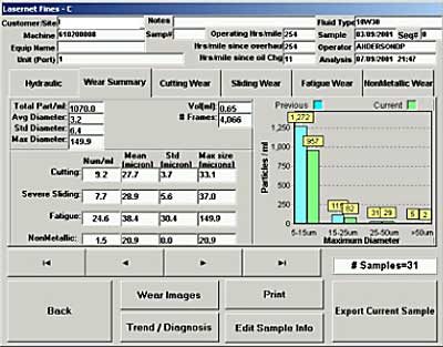
Figure 7a. LNF-C Wear Summary Screen 254 Hrs
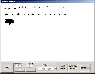
Figure 7b. LNF-C Particle Image Map
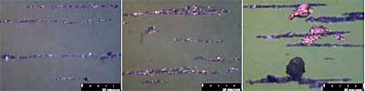
Figure 7c. Photographs showing fine rubbing wear during normal running
Sample C – 366.7 Engine Hours - Normal Running (Mild Wear)
The LNF-C wear summary result after 366.7 hours of operation is shown in Figure 8a. The total number of particles greater than 4 ìm detected and counted was still very low and down to 745/ml. The number of particles that were greater than 20 um was negligible as shown in the cutting, severe sliding, fatigue and non-metallic wear categories. The LNFC image map of particle silhouettes for these particles is shown in Figure8b. As with sample B, these results coincide with normal wear modes and one would expect a reduction in wear particles after the break-in period and several oil changes. The ferrograms, Figures 8c, also confirm a majority of normal rubbing wear particles with the occasional larger particle.
Spectrometric oil analysis of sample C, as shown in Figure 5, confirms the low concentrations of wear metals.
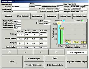
Figure 8a. LNF-C Wear Summary Results
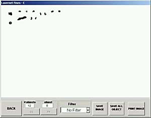
Figure 8b. LNF-C Particle Image Maps
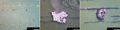
Figure 8c. Photographs showing fine rubbing wear and the occasional larger particle
Sample D – 411.3 Engine Hours – Beginning of Wear Out
The LNF-C wear summary result after 411.3 hours of operation is shown in Figure 9a. The total number of particles greater than 4 ìm detected and counted has increased by more than a factor of 10 and is up to 11,367/ml. The number of particles that were greater than 20 ìm has also increased dramatically as shown in the severe sliding, fatigue and non-metallic wear categories. The LNF-C image map of particle silhouettes for these particles is shown in Figure 9b. The LNFC results confirm an increase in the wear process that is also substantiated by the ferrograms prepared from this sample. When compared to samples B and C, there is a considerable increase in fine rubbing wear, Figure 9c, with more frequent occurrences of large sliding and fatigue wear particles.
Spectrometric oil analysis of sample D, as shown in Figure 5, confirms the increased wear mode through increases in the wear metals concentrations of iron, aluminum, copper and silicon.
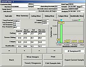
Figure 9a. LNF-C Wear Summary Results
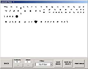
Figure 9b. LNF-C Particle Image Maps
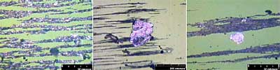
Figure 9c. Photographs showing increased rubbing wear, large severe sliding aluminum particle and large aluminum fatigue flake
Sample E - 534 Engine Hours – Wear Out
The LNF-C wear summary result after 534 hours of operation is shown in Figure 10a. The total number of particles greater than 4 ìm detected and counted has more than doubled and is up to 24,493/ml. The number of particles that were greater than 20 ìm has also increased dramatically as shown in the severe sliding, fatigue and non-metallic wear categories. The increase and large number of fatigue particles is of particular concern. The LNF-C image map of particle silhouettes was electronically filtered to show only fatigue particles, Figure 10b.
Please note that the LNF-C Fines analyzes the outline shape of particles, that is, their” silhouettes”. The results are generated by computing the outlines into a complex Neural-Net pattern recognition algorithm that has been trained using actual known wear particle silhouettes. Cutting wear, fatigue wear and sliding wear particles were manufactured by test apparatus at Swansea University and the collected particles were used to train the LNF wear particle recognition software. Since the optical system within LNF-C uses transmitted light (back lighting), it is not possible for LNF to distinguish particle color, texture or surface attributes. These are important attributes to be considered when making a wear particle type analysis. Hence, the results obtained for each wear category are only those typical of that type of particle when viewed as a silhouette. This is analogous to looking at particles under the optical microscope using only transmitted light.
It should also be mentioned that other types of particles such as molybdenum disulfide, carbon flakes and dark metallo-oxides, should they be present in a sample, will be classified in one of the wear categories of severe, fatigue or cutting depending upon their shape. Any particle that blocks light will be classified in one of the three metallic particle categories, i.e., sliding, fatigue or cutting.
Since this is a reciprocating engine, it is not expected that there would be many surfaces in rolling contact that would be capable of producing true fatigue particles such as found in ball bearings or gear teeth. Instead, the vast majority of particles classified as ‘fatigue’ by the LaserNet Fines simply are not long enough to be classified as sliding wear particles. Examination of the particle surfaces by ferrography reveals that m any particles show surface striations, as in Figures 6c and 8c, even though the particles are not much longer than they are wide. Caution must be used when the LNF-C puts particles in the fatigue category because the LNF-C relies only on the silhouette image.
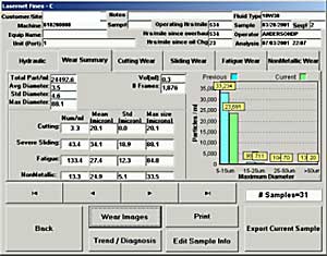
Figure 10a. LNF-C Wear Summary Results
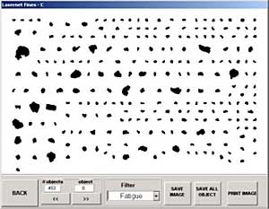
Figure 10b. LNF-C Particle Image Map
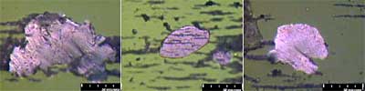
Figure 10c. Photographs showing large fatigue particles
The wear out process has definitely increased and spectrometric oil analysis of sample E, as shown in Figure 5, also confirms the increased wear mode through increases in the wear metals concentrations of iron, aluminum, copper and silicon. Although the spectrometric technique is incapable of volatilizing, and thus analyzing the large wear particles as detected by LNF-C and ferrography, sufficient smaller wear particles are also generated to provide a qualitative and quantitative analysis of the actual metals causing the wear process.
Discussion
The LNF-C results were found to be extremely consistent in terms of both the quantitative and qualitative aspects of more traditional techniques, namely ferrography and spectrometric analysis. The LNF-C’s shape recognition feature showed a substantial increase in both fatigue and severe sliding debris during break-in and the final hours of engine operation. Although it is impossible to ascertain the nature and source of the debris by this method, it certainly would warrant a detailed ferrographic analysis by an expert analyst.
The ferrographic analysis of 5 samples clearly shows how well both the overall particle counts and the more detailed particle types compare with the LNF-C results. The aluminum particles can easily be identified by ferrography because they are nonferrous. Unlike ferrous particles, nonferrous materials will be randomly deposited down the length of the ferrogram and not necessarily with their longest edge leading across the width of the ferrogram. The particles also appear very bright in comparison with the other debris as can be seen by some of the particle images presented in this report.
The spectrometric analysis of the samples was made more difficult by the unusually high frequency of oil changes; however, trends of wear metals that coincide with LNF-C data and ferrography throughout the test were still evident. Good correlation was obtained to confirm increased wear during break-in, reduced wear during the normal operation and again increased wear towards engine wear out. The limitations of atomic emission spectroscopy to accurately quantify wear metal concentrations above 10 ìm in size was also shown not to be a detriment in predicting wear modes.
Conclusion
It is not feasible to make ferrograms and analyze each and every sample because ferrography is both time consuming and expensive. This report has demonstrated how both the automatic particle shape classification and atomic emission spectroscopy can be used in conjunction with each other and applied as screening tools for selective ferrography analysis. The LNF-C can complement ferrography by taking away the subjectivity and automating it to a point where more detailed analysis is warranted. Atomic emission spectroscopy can provide the elemental analysis trend and information necessary to help pinpoint the cause of the wear process so corrective action can be taken to avoid unexpected failure.

This information has been sourced, reviewed and adapted from materials provided by AMETEK Spectro Scientific.
For more information on this source, please visit AMETEK Spectro Scientific.