A quadrupole mass filter is composed of four mutually parallel, highly precise, electrically-isolated electrodes. The orientation of the electrodes is such that there is a hyperbolic (quadrupolar) electric field between them. The common quadrupole fabrication technique involves positioning the four round poles in such a fashion that the centers of the poles coincide with the corners of an imaginary square.
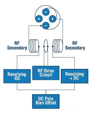
Figure 1. Schematic of typical quadrupole power supply connections
The application of a combination of precise DC and RF voltages to the quadrupole rods helps focusing the ions to be mass analyzed down the quadrupole center. For a specific system, the amplitude of the voltages identifies the mass or range of masses that have stable trajectories through the quadrupole. Striking the quadrupole electrodes neutralizes the ions with unstable trajectories. Two electrical connections are required for the quadrupole. Schematic of a typical quadrupole power supply connections is illustrated in Figure 1.
Mathieu Equation
When discussing quadrupole theory, it is customary to mention the Mathieu Equation:
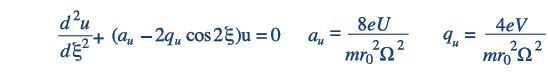
In the above equations, u= Position along the coordinate axes (x or y) and is represented as Ωt/2, in which t is time and Ω is the applied RF frequency; e = the charge on an electron; U = Applied DC voltage; V = Applied zero-to-peak RF voltage; m = Mass of the ion; and r0= The effective radius between electrodes. The solution to this second order linear differential equation is as follows:
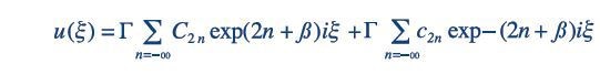
The aforementioned equation is intuitively reduced to a similar infinite sum of sine and cosine functions. Considering ion trajectories as infinite sums of sine and cosine functions, with each succeeding term comprising higher frequency and smaller amplitude, is acceptable. This represents that in each of the x and y direction, the motion is sinusoidal, comprising micromotion at the harmonic frequencies added in and macromotion at the fundamental frequency (ξ 0).
Graphing the Solution
Graphical treatment can answer the questions such as ‘Does the ion have a stable trajectory at the voltages applied? Will the ion pass through the quadrupole?. The families of solution boundaries for the Mathieu equation that lie near the origin are depicted in Figure 2, showing four distinct regions of stable trajectories for ions passing through the quadrupole, utilizing the Mathieu a and q parameters. The traditional operating region for quadrupole mass filters is represented by the Region A in Figure 2.
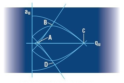
Figure 2. The Mathieu stability diagram in two dimensions (x and y). Regions of simultaneous overlap are labeled A, B, C, and D.
The amplified view of this First Stability Region is illustrated in Figure 3, showing suitable substitutions for the Mathieu parameters a and q to translate the axes into RF-DC voltage space for m/z 219. The r0 is computed based on a round quadrupole rod diameter of 9.5mm and an operating frequency of 1.2MHz. The area inside the boundaries characterizes voltages with stable trajectories, while the the area outside the boundaries characterizes unstable trajectories for that stability region.
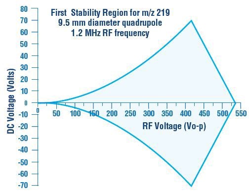
Figure 3. Expanded view of region “A” from Figure 2 (the ‘First Stability Region’)
Constant Resolution Scans
The top halves of the stability diagrams for multiple masses plotted in the same RF-DC space is illustrated in Figure 4. The bottom portion of Figure 4 indicates the ion current that would be quantified when scanning RF and DC voltages through the values along this scan line as a function of time. If ions of different masses are directed into the entrance of the quadrupole, only some ions will traverse the quadrupole to reach the detector at the exit. This relies on whether the voltages yield stable trajectories.
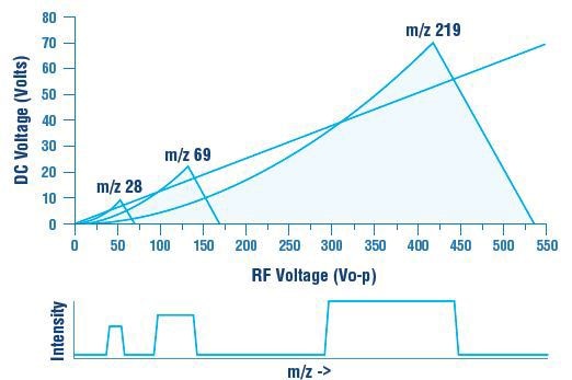
Figure 4. Stability diagrams for m/z 28, 69 and 219 plotted in RF-DC space, showing a straight scan line through the origin.
Decreasing the slope of the mass scan line(dotted scan line in Figure 5) allows the scan line to pass through a major area of the stability diagram. This, turn, widens the mass peak. The outcome of this characteristic shape of the stability diagram is that, as the resolution is reduced (making the peak wider), the position of the leading edge of the mass peak moves to lower apparent mass three times quicker than the trailing edge of the mass peak moving to higher apparent mass. This moves the mass peak center to lower apparent mass.
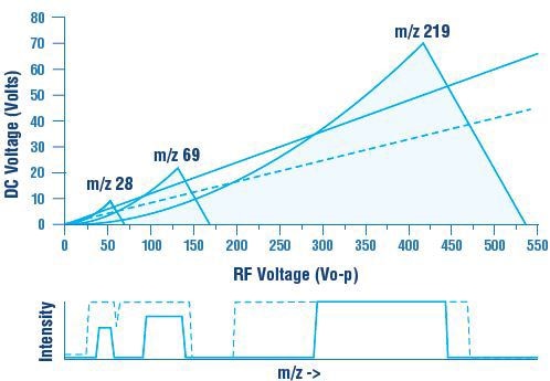
Figure 5. When the slope of the scan line is reduced, the mass peaks widen, with the center of mass position moving to lower apparent mass.
Experimental mass scans at two resolutions demonstrating this effect is depicted in Figure 6.
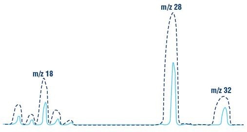
Figure 6. Experimental mass scan from m/z 15 to 35 demonstrating two different mass resolutions.
Unit Mass Resolution Scans
Commercial quadrupoles are typically operated with a mass resolution rather than a constant resolution mode. The mass resolution linearly increases with rising mass such as unit mass resolution, or constant peak width. The scan line passing through the origin needs to be a curve with an increment in the DC/RF voltage ratio with increasing mass in order to obtain unit mass resolution throughout the mass range (Figure 7).
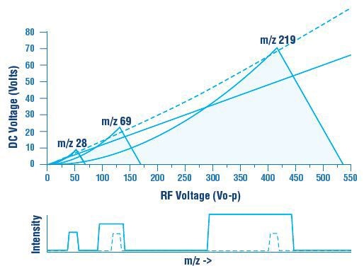
Figure 7. In order to achieve constant peak width across the mass range, a scan line that goes through the origin must be a curve with an increase in the DC to RF voltage ratio with increasing mass.
Traditionally, approximation of this curved ideal scan is done utilizing a straight line in analog hardware by raising the slope of the scan line and lowering its intercept such as it won’t pass through the origin (Figure 8).
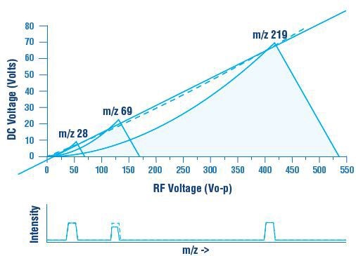
Figure 8. In order to achieve constant peak width across the mass range, a scan line that goes through the origin must be a curve with an increase in the DC to RF voltage ratio with increasing mass.
In Process Insights systems, the intercept that largely influences low mass resolution is termed as delta-M and the slope of the scan line that largely influences high mass resolution is termed as delta-Res. The ‘error function’ that characterizes the deviation between the ‘ideal’ curved scan function and the straight line approximation has been put into practice in commercial systems (Figure 9). Such an analog correction circuit is traditionally called the ‘linearizer’ circuit by Process Insights.
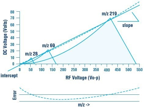
Figure 9. The ‘error function’ that represents the difference between the straight line approximation and the ‘ideal’ curved scan function has been implemented in commercial systems.
Conclusion
This graphical approach helps understanding quadrupole operation intuitively without exploring the equations of motion extensively. Traditional summaries of quadrupole theory give the wrong impression that quadrupoles are operated with constant resolution and constant a/q ratios. Conversely, commercial quadrupoles typically employ some electronic or software implementation for approximation of the curved scan function defined by physics to give unit mass resolution.

This information has been sourced, reviewed and adapted from materials provided by Process Insights - Mass Spectrometry.
For more information on this source, please visit Process Insights – Mass Spectrometers.