Sponsored by EDAXFeb 1 2023Reviewed by Olivia Frost
The process of analyzing geological and extraterrestrial materials through Scanning Electron Microscope (SEM) imaging and Energy Dispersive Spectroscopy (EDS) mapping typically entails the use of high magnifications.
This approach is necessary to examine microscale features and to obtain a representative area of the sample, while also minimizing the impact of variations in grain size and phase distribution.
A key feature of APEX™ is Montage Large Area Mapping, which allows for detailed large-area imaging and EDS, as well as Electron Backscatter Diffraction (EBSD) mapping. This is achieved by utilizing stage movements to collect high-resolution images and maps through a grid pattern over a large surface area of the sample, and then stitching them together to create a montage.
Experiment
To demonstrate the capabilities of the Montage Large Area Mapping feature in APEX, a 2.5 x 1.5 cm section of the Hornblende Basalt Porphyry was selected as the sample. This specimen displays a porphyritic texture, featuring phenocrysts embedded within a matrix of plagioclase, orthopyroxene, Fe-Ti oxides, and apatite.
The data was collected utilizing a field emission SEM equipped with an EDAX Octane Elite Super Silicon Drift Detector. EDS maps were generated in a 24 x 27 grid across the entire section, which was then automatically aligned and stitched together to create a 6144 x 5619-pixel montage of maps, using the APEX Montage Large Area Mapping feature (Figure 1).
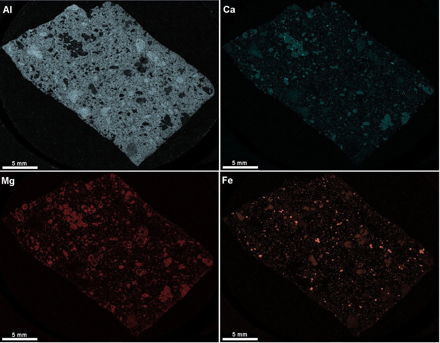
Figure 1. Montage EDS maps of an entire 2.5 x 1.5 cm Hornblende Basalt Porphyry section acquired using APEX 2.0 software. Image Credit: EDAX.
The Montage Large Area Mapping feature in APEX is designed to help users easily create montages of maps using a simple setup wizard. It guides the user to move the stage to the starting position to collect the top-left image, then to the ending position to collect the bottom-right image. Once the images are collected, the number of fields is automatically calculated, and a visual representation of the montage layout in a grid format is presented.
The position marks, located at the top left and bottom right of the images, can be adjusted by the user to set the starting and ending positions. As a result of this alteration, the number of fields is recalculated. The Preview Image feature, in addition, scans the montage and compiles an image of each field.
The user can adjust the starting and ending positions, and preview the alignment before the mapping process. The user can also adjust the matrix size, dwell time, and frames to complete the setup wizard, and the estimated time duration and required disk space are updated accordingly.
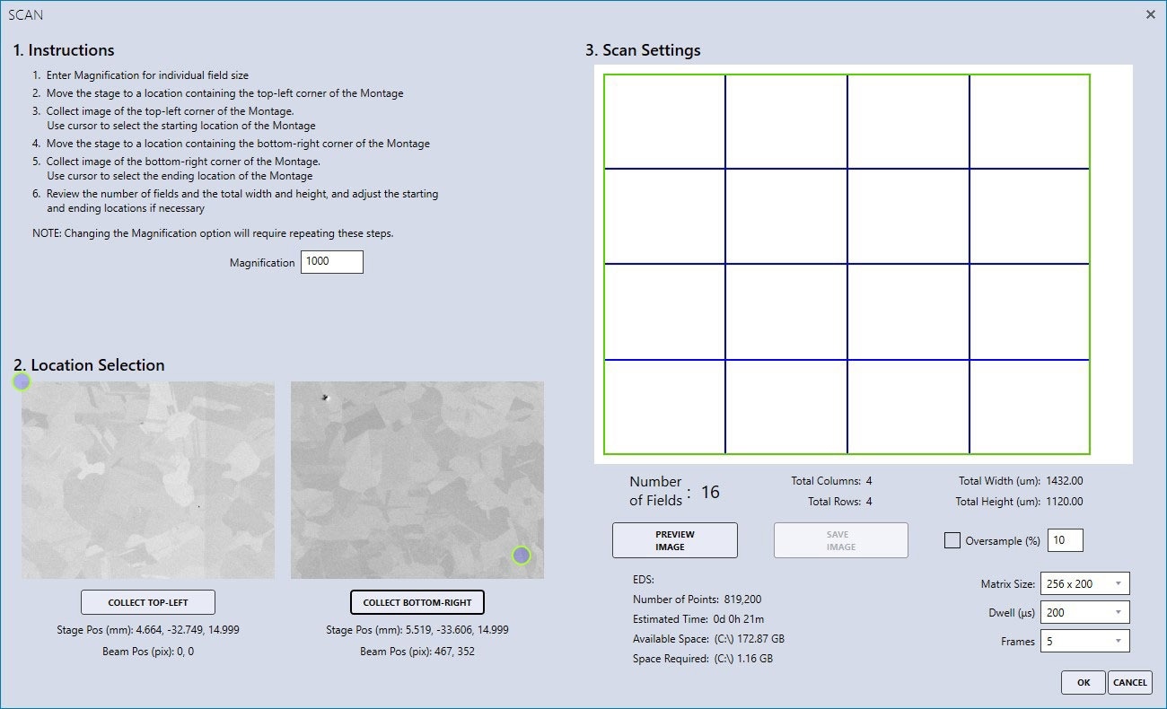
Figure 2. Setup Wizard for Montage Large Area Mapping. The green circle symbols are position marks that can be moved around to adjust the number of fields showing on the right side of the wizard. Image Credit: EDAX.
The Montage Large Area Mapping feature in APEX is similar to standard EDS mapping. The user has the option to lock the Element List before live acquisition or to let the software determine the element list automatically based on a preview spectrum. The preview spectrum is based on the first field in the montage, and the Element List can be modified as desired after the spectrum collection.
In the Review Mode, the user can review the automatically stitched montage maps and individual fields. The user can also export full-resolution data images via the Send to Folder function. Additionally, montage maps can be rebuilt to add or remove element maps.
Proper alignment of edge features of images and maps with respect to neighbors is a basic requirement. Rotation and magnification reference of SEM image scan are major considerations for montage image alignment.
A Transmission Electron Microscope square grid sample was used for adjusting alignment. A montage of SEM images, including multiple square grids, was captured in a 2 x 2 stage field pattern before and after each fine-tuning for evaluating alignment.
The squareness of the grids, along the axes of the four quadrants, which are the boundaries between individual images within the montage, can be analyzed to identify any offsets. These offsets can then be employed as a reference point for making adjustments to the scan rotation and magnification settings.
When the beam axis is not accurately aligned with stage movement in the X-axis, movement along the X-axis also causes a change in position in the Y-axis. This can be observed in the montage of square grids in Figures 3a and 3b. Adjustment of scan rotation is necessary until the discrepancy is resolved (Figure 3c).
Adjusting the rotation offset between the stage and beam is typically done by a skilled service technician, but some SEM software also includes a scan rotation feature that can be adjusted by the user. After the scan rotation is adjusted, it is essential to fine-tune the magnification reference width and height values in APEX or the scan generator software so that the stage moves precisely one field in the X and Y directions.
The process can begin by addressing the direction that requires the most adjustment. To help identify and fix minor offsets, measure the length of the grids along the axes on the screen. It is also worth noting that the SEM image width and stage movement may not be fully calibrated, and the offset may vary with magnification. If the stage moves too short or too far, the reference value is likely too small or large.
Figures 3d-3f illustrate such an adjustment. For EDS mapping, the scale bar on the SEM is not necessarily calibrated along with the stage. The magnification reference adjustment on the EDS side is used to compensate for X/Y scaling. However, for large-area imaging on the SEM side, scale bar calibration is still necessary.
Adjustments to scan rotation and magnification reference are interactive and may need to be repeated multiple times until an optimal alignment for the montage is achieved.
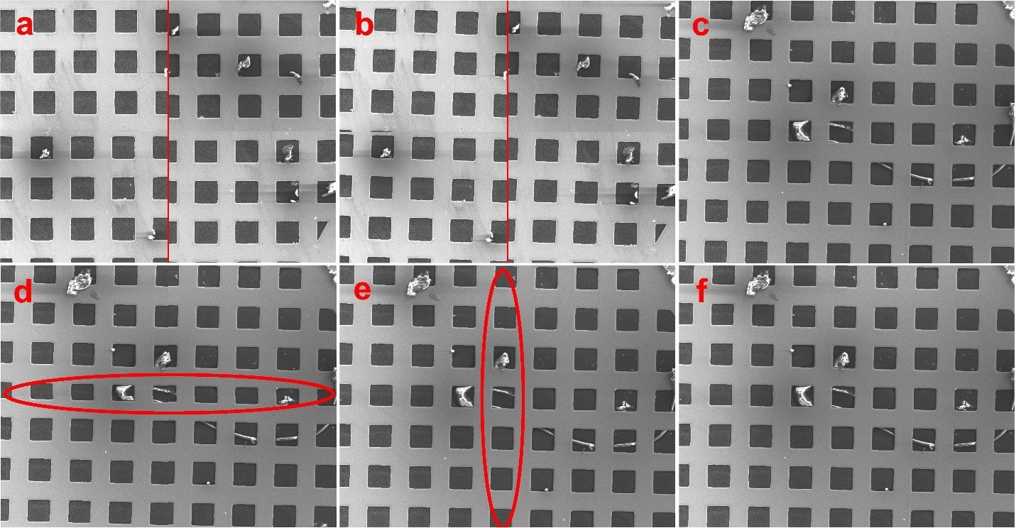
Figure 3. Montage image alignment. The scan rotation angles in a, b, and c are 3º, 1º, and 1.6º, respectively. 1.6º represents a good scan rotation calibration without a mismatch in the figure. d) The stage movement is too far in the Y direction since the grids along the horizontal axis are heavily shrunk in the Y direction. e) After decreasing the reference height value, the stage moves exactly one field in the Y direction. The stage still moves a little far in the X direction as the horizontal side of the grids along the vertical axis is measured slightly shorter than the vertical side. f) Magnification reference adjustment is done after marginally decreasing the reference width value. Image Credit: EDAX.
It is possible to adjust the focus with the working distance or Z stage movement, but it is recommended to maintain a constant working distance throughout the entire imaging/analyzing area to minimize errors. To accomplish this, the sample should be polished flat and mounted parallel to the stage motion.
It is essential to ensure that the X-Y motion of the sample or stage is perpendicular to the beam axis. The tilt, a vector that is perpendicular to the surface of the sample, should be evaluated.
In this example, three positions at the edge of the stage of a field emission SEM were selected, and the stage coordinates (x,y,z) P0 = (-31.5413, 17.5088, 60.4446), P1 = (2.7049, -36.4853, 60.4993), and P2 = (32.7951, 14.9375, 60.3005) (in millimeters) were recorded.
The Z of each position was determined by using Z stage motion only to focus a spherical dirt particle with a diameter of approximately 500 nm on the stage at 20,000 X magnification. Following the method described by Ritchie et al. 1, the tilt is:
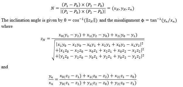
Equation 1.
It was determined that a maximum variation in the Z axis of 0.2 mm was observed, indicating a slight inclination of the stage at 0.2 degrees at an orientation of ϕ = 46.9 degrees. It is important to note that when a flat sample is not mounted parallel to the stage, adjustments in rotation and tilt can be made to ensure that the surface is perpendicular to the beam.
Conclusion
APEX Montage Large Area Mapping offers powerful large area mapping capability. Additionally, they illustrate that the proper alignment is crucial for seamless montages. The Hornblende Basalt Porphyry section has various phenocrysts with varying grain sizes and distribution. Some conspicuous grains span almost the entire field of view at low magnification.
For this type of application, the Montage Large Area Mapping option can be used to map a representative area, which can lead to a more precise calculation of the bulk composition.
Reference
- N.W.M. Ritchie et al., Forensic Chemistry 20 (2020) 100252

This information has been sourced, reviewed, and adapted from materials provided by EDAX.
For more information on this source, please visit EDAX.