Within this experiment, a K-Alpha™ X-ray Photoelectron Spectrometer (XPS) System from Thermo Scientific™ was utilized to inspect a tarnished aluminum component.
Using X-ray photoelectron spectroscopy (XPS) in this instance meant that the identification and quantification of chemical disparities between optically distinct areas on the sample were achievable.
Introduction
Undertaking sample analysis via XPS is often a complex process, with users needing a high skill level to properly load samples, efficiently collect data, and thoroughly interpret the results.
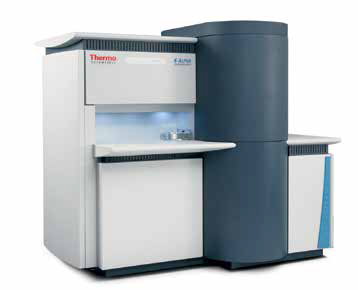
Thermo Scientific K-Alpha XPS.
The K-Alpha surface analysis system allows researchers to use this potent analytical system via a unique combination of intuitive software and efficient hardware design, with no compromise in performance or information content.
The Thermo Scientific Avantage software is used to control the K-Alpha system, controlling every aspect of the sample’s analysis. Safe sample transfer protocols, working alongside a point-and-shoot user interface via live camera views allow for fast, straightforward sample loading, navigation and analysis alignment.
When this, already user-friendly, the operation is combined with robust, integrated analytical tools such as ‘Survey ID’, ‘Multi-spectrum insert’, and full peak deconvolution, an XPS point analysis is relatively simple to perform.
This article documents the use of the K-Alpha to analyze a tarnished aluminum part, allowing the user to acquire chemical state information from various regions of the surface, as well as gaining an understanding of the source of discoloration noted on the surface.
Method
First, the sample was mounted onto the 60 mm × 60 mm sample platter using the two supplied spring clips, as shown in Figure 1. The user wore latex gloves in order to prevent any contamination of the platter or sample.
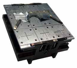
Figure 1. Picture of the aluminum sample mounted on the K-Alpha sample block.
Next, the sample was loaded into the fast entry load-lock, before the button was pressed in the software to pump down and relocate the sample carrier to the analysis chamber. When the pressure in the load-lock reaches an appropriate level, sample transfer occurs automatically.
When samples are loaded into the analysis chamber and the user double-clicks on the platter image, it moves to the position of interest. A point analysis object may be inserted by first selecting ‘Point’ from the drop-down menu, then holding down the ‘control’ key on the keyboard and left-clicking on the live optical view, choosing the desired center of the analysis position (Figure 3).
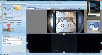
Figure 2. Screenshot of the platter image acquisition, with an inlay of the platter view camera configuration.
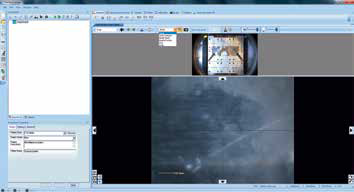
Figure 3. Screenshot of inserting a “Point”.
This process inserts an X-ray object and a point object in the experiment tree (located on the left-hand side of the screen), while simultaneously drawing an ellipse in the optical view. This ellipse represents the size of the X-ray spot in the analysis position (Figure 4).
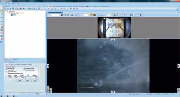
Figure 4. Screenshot after inserting a “Point”.
The X-ray spot’s size dictates the analysis area. This is because the XPS signal is only acquired from the location on the sample irradiated by the X-ray.
The X-ray spot size can be adjusted with the mouse-wheel, allowing it to be adapted to the size of the feature being analyzed. Next, the ‘multispectrum’ tool can be utilized to insert a survey spectrum (Figure 5), allowing the experiment to be run.
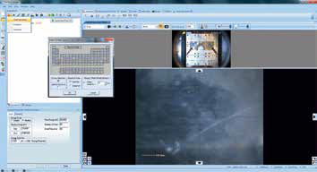
Figure 5. Screenshot of inserting a survey scan using the “Multispectrum insert” tool.
A survey spectrum is a full-range scan which can be employed to identify the elements that exist at the sample’s surface, enabling an elemental quantification to be produced.
While these spectra are generally lower resolution, they do have high count-rates which enables the detection of weaker signals. Additionally, it allows detection of unanticipated elements, so these spectra are used to locate every element present before the collection of high-resolution, region spectra begins.
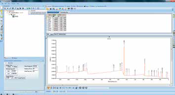
Figure 6. Screenshot of survey scan after “Survey ID”.
Once collected, the survey spectrum is dragged into a processing view and the automated ‘Survey ID’ tool is used to analyze the data via an elemental fingerprinting algorithm. The results of this, including the elemental quantification table, are shown in Figure 6.
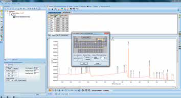
Figure 7. Screenshot of using the “multispectrum” tool to insert region scans.
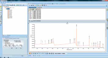
Figure 8. Screenshot after inserting region scans.
Once the results of the survey spectrum analysis are available, these can inform region scans. Region scans can be inserted via the ‘Multi-spectrum insert’ tool, and this is done by clicking on the required elements in the periodic table (Figure 7 and Figure 8). This approach lets the user set up appropriate region scans without the need for knowledge of individual peak positions or other acquisition parameters.
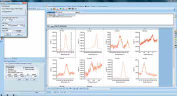
Figure 9. Screenshot of adding peaks to a spectrum.
Once the experiment has finished, region scans may be dragged into a processing view for quantification. This can be done by either adding or fitting peaks. To add peaks, the range cursor must be placed at either end of the peak before clicking the ‘Add peak’ tool. This will then integrate the whole peak area between the data and the selected background type (Figure 9).
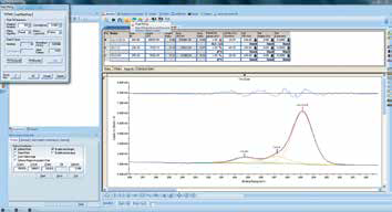
Figure 10. Screenshot of fitting peaks to a spectrum.
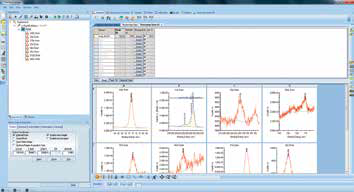
Figure 11. Screenshot of full chemical state quantification after all spectra have been analyzed.
A peak fit may be necessary to deconvolve overlapping peaks from different chemical states. This can be achieved by selecting the range and then using the ‘Peak fit’ tool to add and fit peaks to the spectrum (Figure 10). When every region scan has been processed, the full chemical state quantification can be viewed via the peak table above the spectra (Figure 11).
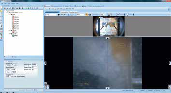
Figure 12. Screenshot of the experiment tree setup to run multiple point analyses.
It is possible to repeat this whole process in order to obtain multiple point analyses within one experiment. Figure 12 illustrates the experiment setup needed to run three consecutive point analyses in the grey, brown, and shiny areas of the sample.
It is also possible to configure the software to automatically run this process via Auto-Analysis mode. In this mode, the experiment is created on-the-fly using the instrument based on an analysis of the survey spectrum. This data can then be exported to a Microsoft® Word® document.
Results
Table 1 is a comparison table of the chemical state quantification, showing each of the three analysis points.
Table 1. Full chemical state quantification for all three analysis points.
| Name |
Shiny Area
At. % |
Grey Area
At. % |
Brown Area
At. % |
| Al2p Al2O3 |
20.11 |
21.38 |
8.64 |
| Si2p SiO2 |
0.36 |
0.23 |
0.60 |
| S2p sulfate |
0.60 |
0.40 |
0.23 |
| Cl2p organic |
0.25 |
0.32 |
0.46 |
| C1s C-C/C-H |
17.78 |
9.51 |
11.88 |
| C1s C-O |
11.43 |
13.36 |
10.31 |
| C1s C=O |
3.01 |
2.70 |
2.63 |
| N1s organic |
0.75 |
0.55 |
0.59 |
| O1s |
45.10 |
51.08 |
53.57 |
| Fe2p Fe2O3 |
0.27 |
0.18 |
10.14 |
| Zn2p3/2 ZnO |
0.16 |
0.18 |
0.82 |
| Na1s |
0.18 |
0.12 |
0.14 |
Here, the quantification confirmed that the shiny and grey areas have chemistries which are similar, with the only obvious differences being the levels of carbon and oxygen present. The brown area contains more than 10% Fe2O3 and a substantial increase in the amount of ZnO in comparison with the two other analysis points.
Because the iron oxide is present on the surface, there is a reduction in the signals from the elements below this - particularly aluminum. Attenuating the substrate signal enables the thickness of the iron oxide layer to be calculated via a different tool in the Avantage™ data system, built on a basic two-layer model.
By using this tool, the iron oxide thickness was determined to be 1.5 nm. By identifying the heightened levels of iron oxide and zinc oxide, the analyst was able to ascertain the cause of the sample’s discoloration and therefore the failure of the component.
Summary
It is possible to use the K-Alpha XPS system to analyze points of interest on the surface of a sample rapidly, effectively, and reliably. This is due to the user-friendly experiment setup interface, coupled with the integrated data-processing tools.
Acknowledgments
Produced from materials originally authored by Chris Baily and Tim Nunney from Thermo Fisher Scientific.

This information has been sourced, reviewed and adapted from materials provided by Thermo Fisher Scientific – X-Ray Photoelectron Spectroscopy (XPS).
For more information on this source, please visit Thermo Fisher Scientific – X-Ray Photoelectron Spectroscopy (XPS).