In order to devise an approach to identify around 30 different metals and trace elements in waters, wastewaters and solid wastes by ICP-OES, the U.S. EPA produced Method 200.7.1
Established in 1994, Method 200.7 has been routinely performed in environmental labs across the United States.
With the continual expansion of industry, pollution and wastes are persistently produced in larger quantities, leading to an increasing number of samples, which necessitate analysis per Method 200.7.
In an attempt to meet the needs of increasing demand, PerkinElmer’s Avio® 560 Max entirely simultaneousICP-OES includes an integrated High Throughput System (HTS) for high-speed sample-to-sample times.
The HTS is a valve-and-loop system that significantly reduces the time needed for the sample to reach the nebulizer and washout time post-analysis by utilizing a vacuum to both quickly fill and wash the sample loop.
This work outlines the analysis of wastewaters following Method 200.7 utilizing the Avio 560 Max ICP-OES and advancing on previous work.2
Experimental
Samples and Sample Preparation
Development and evaluation of the methodology were achieved with four separate wastewater certified reference materials:
- Wastewaters C, D and H (High Purity Standards™, Charleston, South Carolina, USA)
- WasteWatR™, Trace Metals (ERA, Golden, Colorado, USA)
These standards were provided as concentrates and diluted in accordance with the certificate instructions. Samples were prepared in line with Method 200.7: 50 mL were acidified with 2 mL of 1:1 HNO3 and 1 mL of 1:1 HCl, then stationed in a hot block and heated to a temperature of ≈ 85°C.
The solutions were taken out with ≈ 20 mL final volume for cooling cool and using deionized water diluted to 50 mL for analysis.
All measurements were taken in opposition to external calibration curves, where the concentrations in Table 1 in 2% HNO3 (v/v) set the standards for preparation.
Table 1. Calibration Standards. Source: PerkinElmer, Inc.
| Element |
Standard 1
(mg/L) |
Standard 2
(mg/L) |
| Ag, Al, As, B, Ba, Be, Cd, Co, Cr, Cu, Fe, Li, Mn, Mo, Ni, P, Pb, Sb, Se, Si, Sn, Sr, Ti, Tl, V, Zn |
0.5 |
1 |
| Na, Mg, K, Ca |
10.5 |
21 |
After preparation in 2% HNO3(v/v), the internal standard (yttrium, Y) was added to the sample stream via a port in the HTS valve. Interelement corrections (IECs) were administered to all measurements.
As detailed in Method 200.7, the IEC solutions were run at the appropriate concentrations, except where they were beyond the linear range. In these instances, the concentrations of the IEC solutions were modified to come within the linear range.
Instrumental Conditions
All analyses were conducted on an Avio 560 Max ICP optical emission spectrometer (OES), utilizing the High Throughput System (HTS)3 for the introduction of samples via an S23 Autosampler.
Parameters and conditions of the instrument are displayed in Table 2, along with the analytical wavelengths, analytes and plasma view modes in Table 3.
Table 2. Avio 560 Max ICP-OES with HTS Instrumental Parameters. Source: PerkinElmer, Inc.
| Paramenter/Component |
Value/Description |
| Sample Uptake Tubing |
Black/Black (0.76 mm id) PVC |
| Internal Standard Tubing |
Green/Orange (0.38 mm id), PVC |
| Drain Tubing |
Gray/Gray (1.30 mm id), Santoprene |
| Nebulizer |
MEINHARD® K1 |
| Spray Chamber |
Baffled Glass Cyclonic |
| Carrier |
2% HNO3 (v/v) |
| Carrier Flow Rate |
0.8 mL/min |
| Sample Loop Volume |
1 mL |
| Injector |
2.0 mm id Alumina |
| Nebulizer Gas Flow |
0.70 L/min |
| Auxiliary Gas Flow |
0.2 L/min |
| Plasma Gas Flow |
8 L/min |
| Torch Depth |
-3 |
| Integration |
Auto |
| Read Time Range |
0.5-5 sec |
| Loop Fill Time |
4 sec |
| Loop Rinse Time |
3 sec |
| Replicates |
2 |
Table 3. Analytes, Wavelengths, and Plasma View Mode. Source: PerkinElmer, Inc.
| Element |
Wavelength (nm) |
Plasma View Mode |
| Ag |
328.068 |
Axial |
| Al |
308.215 |
Radial |
| As |
188.979 |
Axial |
| B |
249.677 |
Axial |
| Ba |
493.408 |
Radial |
| Be |
313.107 |
Radial |
| Ca |
315.887 |
Radial |
| Cd |
214.440 |
Axial |
| Ce |
413.764 |
Axial |
| Co |
228.616 |
Axial |
| Cr |
267.716 |
Axial |
| Cu |
324.752 |
Axial |
| Fe |
238.204 |
Radial |
| K |
766.490 |
Radial |
| Li |
670.784 |
Radial |
| Mg |
285.213 |
Radial |
| Mn |
257.610 |
Axial |
| Mo |
203.845 |
Axial |
| Na |
589.592 |
Radial |
| Ni |
231.604 |
Axial |
| P |
178.221 |
Axial |
| Pb |
220.353 |
Axial |
| Sb |
206.836 |
Axial |
| Se |
196.026 |
Axial |
| Si |
251.611 |
Radial |
| Sn |
189.927 |
Axial |
| Sr |
421.552 |
Radial |
| Ti |
334.940 |
Axial |
| Tl |
190.801 |
Axial |
| V |
292.402 |
Axial |
| Zn |
206.200 |
Axial |
| Y (Internal Standard) |
371.029 |
Axial and Radial |
Conventional sample introduction components and conditions were utilized, including a complete argon flow of 9 L/min. While Method 200.7 asserts that four replicates are necessary, a typical implementation is the use of two or three replicates to improve sample throughput.
To ensure this is more relevant and works for commercial labs, all measurements were taken using two replicates. All analyses were conducted using auto-integration with a read-time range of 0.5-5 seconds, which yielded rapid analysis for high-level analytes while also permitting accurate measurements of low-level analytes.
To streamline analysis, auto background correction was implemented. Under these conditions, sample-to-sample time was in the region 60 seconds.
For optimum performance, auto integration with variable read times was used, which resulted in the sample-to-sample time varying depending on the analyte concentrations in the samples: for higher concentrations, sample-to-sample time will be under 60 seconds; for samples with lower concentrations, the sample-to-sample time can be just over 60 seconds.
To meet conventional operating procedures, three or four replicates can also be applied with minimal sample-to-sample time gain.
Results and Discussion
To ensure compliance with Method 200.7, quality control (QC), the appropriate criteria for sample handling and preparation as well as the instrumental analysis must be satisfied.
The following criteria specifically relates to instrumental analysis and will be evaluated to establish the validity of the Avio 560 Max system: instrument performance checks (IPCs), linear dynamic range, spectral interference checks (SICs), method detection limits (MDLs), stability and accuracy.
Using Smart Software to Facilitate Data Analysis
Syngistix for ICP software (version 5.1 or higher) incorporates many smart features to enable data analysis and interpretation, including smart methods, smart workflow, smart data and smart monitoring.
While all of these were utilized when receiving data for Method 200.7, only a small number of the features will be outlined here.
One of the most crucial aspects of obtaining solid data is reviewing and satisfying good linearity for calibration curves. This can be completed with ease using Data Viewer, as shown in Figure 1.
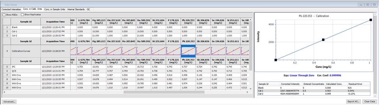
Figure 1. Calibration information displayed in Data Viewer. Image Credit: PerkinElmer, Inc.
When data is obtained using Data Viewer, thumbnails of the calibration curves emerge, which give the user a brief overview. For more in-depth analyses, details of the calibration curve materialize when the thumbnails are clicked.
This shows the correlation equation, coefficients, entered concentrations, corrected intensities and calculated concentrations for each standard, as well as the residual error for each standard.
If modification of the calibration curve is required (for example, if a standard was out of range), the Edit Calibration window displays the same information (Figure 2), which enables editing of the calibration information.
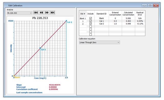
Figure 2. Detailed calibration information displayed in the Edit Calibration window. Image Credit: PerkinElmer, Inc.
When running long-term stability, it is also vital to monitor the stability of the internal standard.
The user is able to monitor the real-time performance of an active run due to the normalization of internal standard response (normalized to the calibration blank) displayed automatically in Data Viewer in real-time (Figure 3).
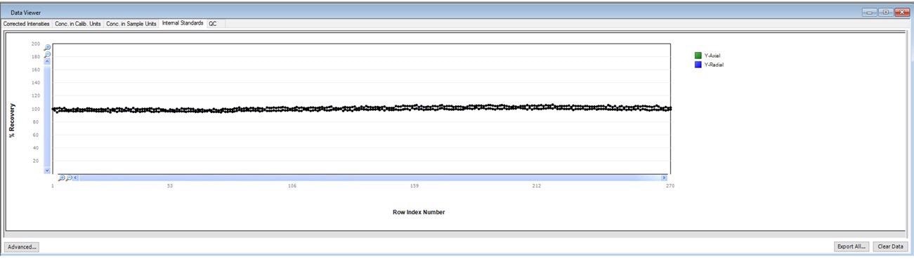
Figure 3. Internal standard plot in Data Viewer. Image Credit: PerkinElmer, Inc.
Initial QC: Initial Performance Check and Quality Control Sample
To substantiate the calibration curve’s quality, an initial performance check (IPC) must be analyzed directly after the calibration. The IPC must be a separate standard made equivalent to the stock standard as the calibration standards.
Additionally, it is necessary to make a quality control sample (QCS) to the same concentration as the IPC, but from a second-source standard to verify the concentration of the stock solutions utilized for the calibration standards.
Recover within 5% of their true values for both the IPC and QCS are required for the analysis to proceed.
For this assessment, all elements were present at 0.75 ppm, with the exception of the minerals (Ca, K, Mg, Na), which were added at 21 ppm. Figure 4 demonstrates that both the QCS and IPC recovered within the 5% needed for all analytes.
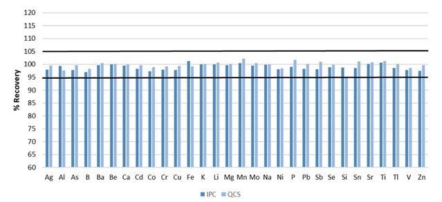
Figure 4. Recoveries for initial IPC and QCS. Image Credit: PerkinElmer, Inc.
Method Detection Limits
Method 200.7 details that method detection limits (MDLs) are established by measuring a standard seven times which has been contaminated with analytes at 2-3 times the instrumental detection limits (IDLs).
Multiplication by 3.14 of the mean deviation of the seven measurements is carried out to obtain MDLs at the 99% confidence level. The IDLs must be established prior to measuring the MDLs can be measured. IDLs were calculated by multiplying the standard deviation of 10 blank measurements by three.
Figure 5 illustrates the MDLs plotted beside the certified analyte concentrations in the four reference materials as analyzed in this study. (Note: not all analytes were held in the reference materials.)
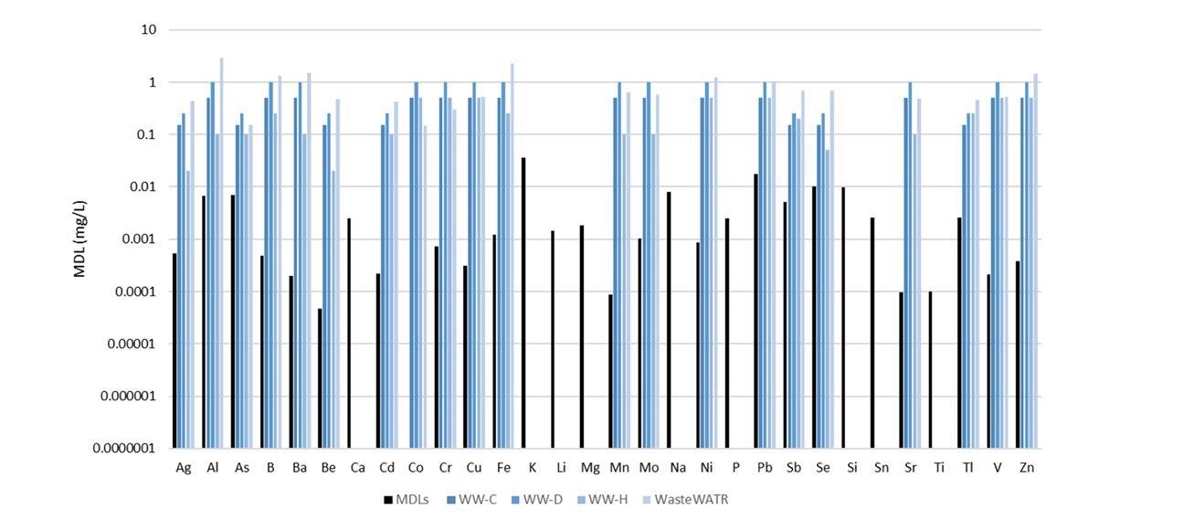
Figure 5. Method detection limits (black) along with certified concentrations in four reference materials (shades of blue). Not all analytes were certified in the reference materials. Image Credit: PerkinElmer, Inc.
The MDLs are considerably lower than the certified values, demonstrating the capacity of the methodology to measure low-level analytes in wastewaters with ease.
Linear Dynamic Range
Method 200.7 declares the linear dynamic range as the highest concentration, which recuperates within 10% of its true assigned value as measured against the calibration curve utilized for analysis.
All linear dynamic range measurements were conducted in multi-element solutions to ensure relevance to sample analyses, which are, in any case, multi-element solutions.
As Table 4 demonstrates, the highest concentration analyzed for most elements is the linear dynamic range. This is representative of the highest concentrations typically found in wastewaters, not the limit of the Avio 560 Max ICP-OES.
Table 4. Linear Dynamic Range. Source: PerkinElmer, Inc.
| Elements |
Linear Range (mg/L) |
| Cd, Mn, Sr |
30 |
| Ba |
40 |
| Co, Cr, Ni, Sn, Ti, Tl |
50 |
| Be |
70 |
| Ag, Al, As, B, Cu, Fe, Li, Mg, Mo, P, Pb, Sb, Se, Si, V, Zn |
100* |
| Ca, K, Na |
500* |
*= highest concentration evaluated
The linear range of the Avio 560 Max can be further extended, if necessary, by choosing less sensitive wavelengths, modifying the plasma viewing mode (i.e., axial/radial), switching the viewing height in the plasma to radial mode, varying the torch position, utilizing high-resolution mode and/or using a less sensitive sample introduction system.
Accuracy
With the base characteristics of the methodology determined, the accuracy was established via analysis of four reference materials, whose certified values are exhibited in Table 5. The analyte recoveries for each of the certified elements are shown in Figure 6.
Table 5. Certified Values in Wastewater Reference Materials (all units in mg/L) . Source: PerkinElmer, Inc.
| Element |
Wastewater C |
Wastewater D |
Wastewater H |
WasteWATR |
| Ag |
0.15 |
0.25 |
0.02 |
0.444 |
| Al |
0.5 |
1 |
0.1 |
2.91 |
| As |
0.15 |
0.25 |
0.1 |
0.151 |
| B |
0.5 |
1 |
0.25 |
1.33 |
| Ba |
0.5 |
1 |
0.1 |
1.5 |
| Be |
0.15 |
0.25 |
0.02 |
0.468 |
| Cd |
0.15 |
0.25 |
0.1 |
0.430 |
| Co |
0.5 |
1 |
0.5 |
0.147 |
| Cr |
0.5 |
1 |
0.5 |
0.302 |
| Cu |
0.5 |
1 |
0.5 |
0.526 |
| Fe |
0.5 |
1 |
0.25 |
2.25 |
| Mn |
0.5 |
1 |
0.1 |
0.636 |
| Mo |
0.5 |
1 |
0.1 |
0.578 |
| Ni |
0.5 |
1 |
0.5 |
1.21 |
| Pb |
0.5 |
1 |
0.5 |
1.05 |
| Sb |
0.15 |
0.25 |
0.2 |
0.693 |
| Se |
0.15 |
0.25 |
0.05 |
0.678 |
| Sr |
0.5 |
1 |
0.1 |
0.489 |
| Tl |
0.15 |
0.25 |
0.25 |
0.461 |
| V |
0.5 |
1 |
0.5 |
0.525 |
| Zn |
0.5 |
1 |
0.5 |
1.46 |
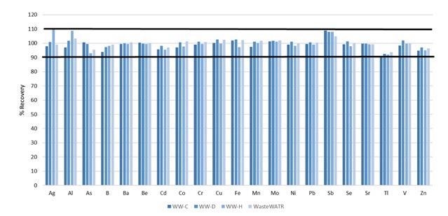
Figure 6. Certified analyte recoveries in four different wastewater reference materials. Image Credit: PerkinElmer, Inc.
With all recoveries within 10% of their certified values, accuracy of the methodology is resolved.
Yet not all the elements detailed in Method 200.7 are certified in the reference materials.
The reference materials were contaminated with these elements, prior to digestion, at the concentrations exhibited in Table 6: their recoveries are shown in Figure 7. All recoveries are within 10%, further establishing the accuracy of the method.
Table 6. Spiked Concentrations of Non-Certified Elements in Wastewater CRMs. Source: PerkinElmer, Inc.
| Analyte |
Concentration (mg/L) |
| Li, P, Si, Sn, Ti |
0.75 |
| Ca, K, Mg, Na |
20 |
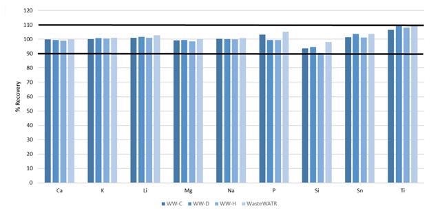
Figure 7. Recoveries of non-certified elements spiked into four wastewater CRMs. Image Credit: PerkinElmer, Inc.
Stability
With the accuracy established, stability was proven by monitoring the recoveries of the IPC standards and measuring wastewater samples, which are run every ten samples.
Figure 8 illustrates how all IPCs over the 4-hour run recover within 10% of their certified values, with a sample-to-sample time of around 1 minute. This demonstrates the excellent stability of the system, despite the quick sample-to-sample time of ≈60 seconds.
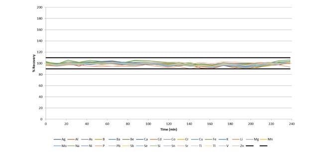
Figure 8. IPC recoveries during a 4-hour run of wastewaters, with a sample-to-sample time of ≈ 60 seconds. Image Credit: PerkinElmer, Inc.
Instrumental design considerations, such as the vertical torch and Flat Plate™ plasma technology, result in exceptional stability while making the most of the dual view capability and consistently moving between axial and radial plasma viewing modes for each sample.
Conclusion
Following the guidelines provided in U.S. EPA Method 200.7, this work illustrates the capacity of the Avio 560 Max ICP-OES to perform high-speed analysis – 60 sec sample-to-sample time – of wastewater.
With reliability, precision, robustness and stability exhibited during the analysis of reference materials and QC checks, the Avio 560 Max ICP-OES with integrated HTS offers a powerful solution for wastewater analysis while utilizing a total argon flow of 9 L/min.
The low argon consumption (9 L/min plasma flow) of the Avio 560 Max ICP-OES enables a swift return on investment for all laboratories, while the HTS considerably reduces sample uptake and washout times in contrast to traditional sample introduction, additionally increasing sample throughput.
References
1. Method 200.7, Revision 4.4: Determination of Metals and Trace Elements in Water and Wastes by Inductively Coupled Plasma- Atomic Emission Spectrometry”, United States Environmental Protection Agency, 1994.
2. “Analysis of Wastewaters Following U.S. EPA 200.7 using the Avio 550 Max ICP-OES”, Application Note, PerkinElmer Inc., 2020.
3. “High Throughput System for ICP-MS/OES,” Product Note, PerkinElmer Inc., 2020.

This information has been sourced, reviewed and adapted from materials provided by PerkinElmer.
For more information on this source, please visit PerkinElmer.