Plastics are widely used polymeric materials employed in a diverse array of applications and across a wide range of popular consumer products.
Polymers used in the production of plastics are typically processed at higher temperatures, working with these in a molten state. Properly comprehending their melting, deformation and flow is central to effectively processing and transforming these into end products.
Polymers are regarded as viscoelastic materials, meaning that they exhibit both viscous (liquid-like) and elastic (solid-like) properties. Their high molecular weight and chemical structure cause polymer melts to exhibit a complicated flow and deformation behavior.
The ability to optimize blends and formulations is dependent on a good knowledge of a polymeric material’s viscoelastic properties. This knowledge is also essential to adapting a process to the properties of a specific material.
A polymer melt’s molecular structure, testing conditions or processing conditions will generally determine whether its viscous or elastic behavior is dominant.
Too much elasticity may result in flow anomalies and undesirable effects during a range of common processing steps,1 for example, a melt stream may swell as it exits the narrow die of an extruder.
Figure 1 displays a series of other examples of flow anomalies resulting from the elastic properties of polymeric fluids.

Figure 1. Typical flow anomalies of viscoelastic polymer fluids. Image Credit: Thermo Fisher Scientific – Materials & Structural Analysis
Two tools frequently employed in the measurement of polymer melt viscosities are capillary viscometers and melt flow indexers. These instruments do not offer any insight into the viscoelastic properties of the tested sample, however.
In contrast, the use of a rotational rheometer with the capacity to perform rheological tests with small oscillatory mechanical excitations can offer users a robust and comprehensive investigation into these properties.
This article offers an overview of the various rheological tests which can be conducted using rotational rheometers. It also outlines how the results of these tests relate to a range of processing conditions and final product properties.
Rotational Versus Oscillatory Testing – The Cox-Merz Rule
Rheology is widely recognized as an excellent tool for the analysis of polymers’ mechanical properties in their various physical states. A number of testing methods can be employed to comprehensively characterize the rheological behavior of polymeric materials.
Rotational steady-state shear experiments offer a means of measuring the non-Newtonian viscosity of dilute and semi-dilute polymer solutions, but the application of an oscillatory shear deformation remains the testing method of choice for polymer melts and solids.
This is because of polymer melts’ high elasticity and their tendency to result in edge failures when exposed to the large deformations typical in a rotational rheometer.
The Cox-Merz rule states that when complex viscosity (Iη*I) is derived from oscillatory frequency sweep measurements plotted against the angular frequency (ω), this will be identical to the steady-state shear viscosity determined via rotational testing plotted against the shear rate.2
The Cox-Merz rule is an empirical rule applicable to a wide range of polymer melts and solutions.
Figure 2 compares viscosity data acquired from rheological tests in rotation versus data acquired in oscillation mode.
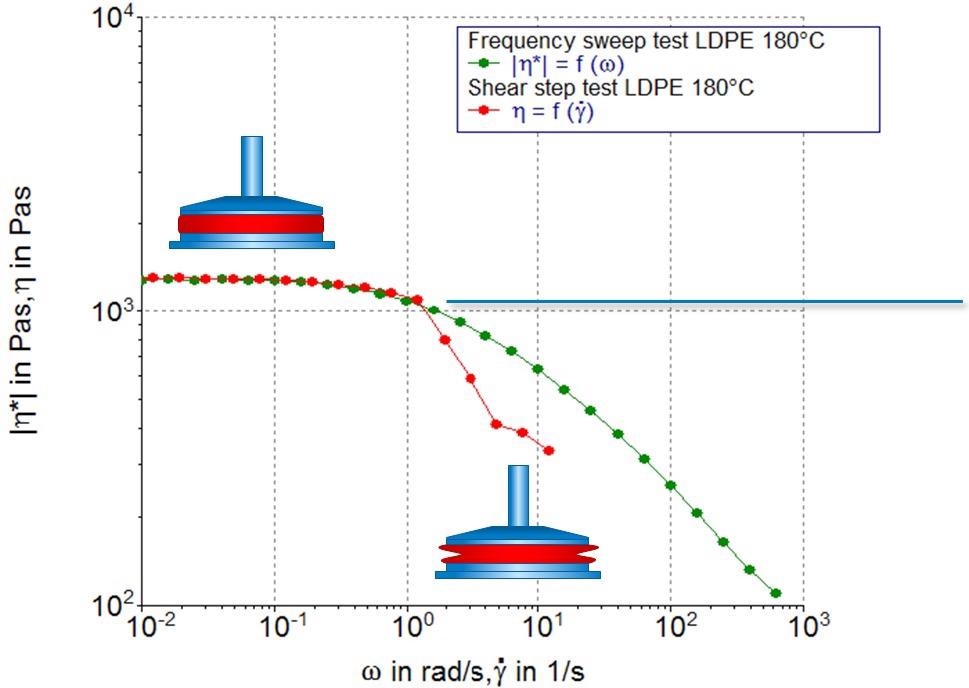
Figure 2. Comparison of viscosity data obtained from a steady state shear (red symbols) and an oscillation frequency sweep test (green symbols). Image Credit: Thermo Fisher Scientific – Materials & Structural Analysis
Viscosity begins to decrease as the end of the Newtonian (zero shear viscosity) plateau is reached. At this point, the shear viscosity (red symbols) drops abruptly and ceases to display a smooth and continuous progression.
This observable drop is the result of sample fracture at the edge of the measuring geometry, a phenomenon caused by secondary flow fields.1 It should be noted that the oscillation frequency sweep (green symbols) provides higher data quality and can accommodate a broader frequency range.
The oscillatory frequency sweep’s enhanced testing range is due to the small amplitudes of the imposed oscillatory shear. Therefore, conducting an oscillatory frequency sweep and applying the Cox-Merz rule is the method of choice when looking to acquire shear viscosity data for polymeric materials.
Using Amplitude Sweep Tests to Identify Linear-Viscoelastic Range
It is important that the applied sinusoidal oscillatory deformation is relatively small and within a material’s linear viscoelastic range (LVR) to ensure that viscosity data from a frequency sweep experiment is comparable.
When maintained within its LVR, the material’s microstructure remains unchanged. Its rheological properties will also remain constant and unaffected by the applied stress of deformation; for example, the storage and the loss modulus (G’ and G’’, respectively) or the complex viscosity.
Should a critical deformation or stress value be reached, this will prompt the material’s microstructure to change, and in turn, its rheological parameters.
To determine the linear viscoelastic range of a material, it is necessary to conduct an oscillation amplitude sweep test. This test must be performed at a constant frequency and involves a gradual increase of the sinusoidal deformation or stress applied by the rheometer.
Results of an amplitude sweep for LDPE at 190 °C are displayed in Figure 2.
In the example presented here, the rheometer software has automatically calculated the end of the linear viscoelastic range of this LDPE melt, determining this to be equal to a deformation of 55%.
It is also advisable to perform additional tests in oscillation mode at a deformation below this critical value, for example, frequency, temperature or time sweep tests. This is unnecessary for tests intended to be outside the LVR, however.
Should it be necessary to perform a frequency sweep test over a wider frequency range of several orders of magnitude, it is advisable to undertake a number of amplitude sweeps at various frequencies to ensure the selected deformation is within the LVR throughout the whole frequency range.
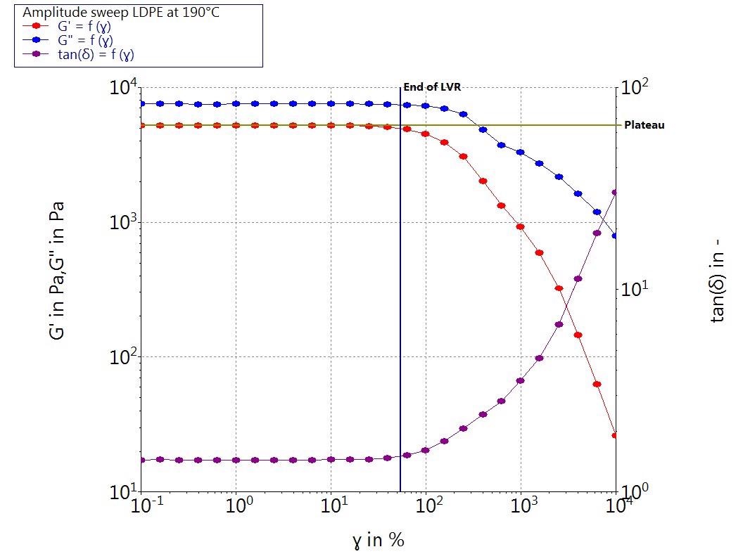
Figure 3. Storage modulus G’, loss modulus G’’ and the complex viscosity Iη*I as a function of the deformation γ for a LDPE melt at 1 Hz and 190 °C. Image Credit: Thermo Fisher Scientific – Materials & Structural Analysis
Using the Frequency Sweep Test to Determine a Material’s Viscoelastic Fingerprint
A diverse array of information can be acquired from performing rheological tests in oscillation mode.
For example, the acquisition of shear rate-dependent viscosity data via oscillatory frequency sweep experiments can be processed using the Cox-Merz rule to quantify a material’s flow resistance during high shear processing applications such as injection molding or extrusion.
In contrast, low frequency/shear data (for example, zero shear viscosity / η0) can be employed to calculate the average molecular weight (Mw) of a polymer melt. This is achieved via the following formula:
Within this equation, the prefactor (k) is dependent on the polymer’s molecular structure.3 Equation 1 is applicable to polymers with a linear chain structure and a molecular weight above a critical value (Mc).
Figure 4 displays an example viscosity curve of a polystyrene melt, highlighting the corresponding shear rate ranges encountered in several routine processing applications.
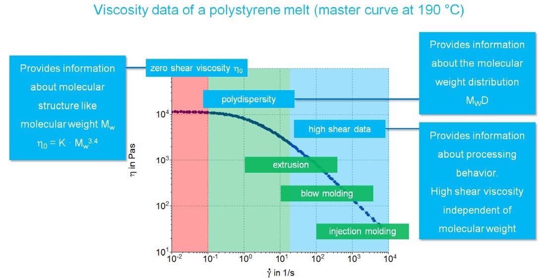
Figure 4. Shear rate depending viscosity of a polystyrene melt and typical applications. Image Credit: Thermo Fisher Scientific – Materials & Structural Analysis
Frequency sweep data also offers a means of directly measuring a polymer’s viscous and elastic properties. These properties are represented by the storage and the loss moduli (G’ and G’’, respectively) and are generally measured at varying frequencies and timescales.
Data from these measurements can illustrate the general structure of a material, alongside valuable information on its molecular weight (Mw) and molecular weight distribution (MWD).
It is possible to employ repetitive frequency sweep measurements over a narrow frequency range to capture the crossover point. This, therefore, enables the detection of thermal degradation, triggering alterations to the MW and MWD.
Figure 5 illustrates an example of this crossover point shifting, highlighting where G’ = G’’ and the MW or MWD differ for an otherwise identical polymer melt.
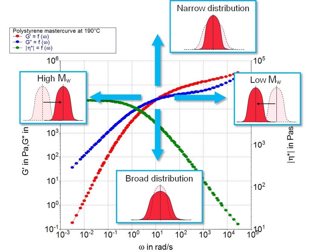
Figure 5. Storage modulus G’, loss modulus G’’ and the complex viscosity Iη*I as a function of the angular frequency ω for a polystyrene melt at 190 °C. Image Credit: Thermo Fisher Scientific – Materials & Structural Analysis
Flow anomalies caused by the elasticity of polymer melts may adversely affect product quality in extrusion and other polymer processing applications.
Figure 6 compares storage modulus data as a function of the applied frequency for a number of polyethylene samples with differing Melt Flow Indices (MFI).
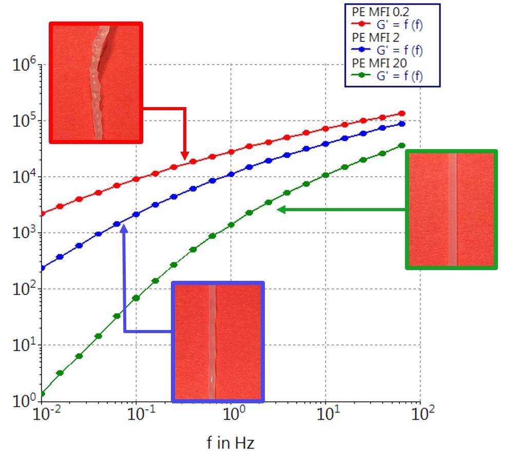
Figure 6. Storage modulus G’ as a function of the angular frequency ω for polyethylene melts with different MFI at 190 °C. The images show the extrusion strands that were prepared with the melts in a twin screw extrusion process. Image Credit: Thermo Fisher Scientific – Materials & Structural Analysis
Each of these three PE samples was processed under identical conditions using a 16 mm parallel twin screw extruder.
Once they reached the end of the extruder barrel, the melts were forced through a vertical rod capillary die with a diameter of 1 mm and an L/D ratio of 10. A laser micrometer was employed to measure the die swell of the extrudate.
A die-swell of 0.5 mm was found to result in a total strand diameter of 1.5 mm for the PE with the lowest molecular weight and highest MFI (~20). The strand exited the extrusion line as an even strand with no observable surface defects (Figure 6).
The PE sample exhibiting medium MFI (~2) displayed an uneven surface structure with a changing diameter, while the PE sample exhibiting the lowest MFI (~0.2) and highest molecular weight displayed obvious indications of melt fracture under the extrusion conditions also utilized for the other samples.
An examination of the rheological data highlights that the three samples are notably different in terms of their elasticity (G’). This is particularly prevalent at the lowest frequency (10-2 Hz), where the values in G’ differ in one or more orders of magnitude.
Storage modulus also offers a sensitive indicator of the elasticity incorporated by a high molecular weight tail.
Figure 7 compares the results of a total of three frequency sweeps performed on a low molecular weight LDPE and two blends of an identical LDPE that also featured a small weight fraction of a high molecular weight PE.

Figure 7. Storage modulus G’ and loss modulus G’’ as a function of the angular frequency ω for a low molecular weight polyethylene melt and two blends at 190 °C. Image Credit: Thermo Fisher Scientific – Materials & Structural Analysis
G’ shows clear differences for these three melts in the low frequency range, and a small fraction of 1 wt% of high molecular weight PE can also be detected.
It should be noted that it is rarely possible to view these small differences when employing Gel Permeation Chromatography (GPC) or related techniques to ascertain molecular weight distribution.
MFI results achieved via a capillary viscometer would also fail to reveal differences between the three samples.
Storage modulus data acquired via oscillatory frequency sweep experiments remains the most sensitive indicator of a high molecular weight tail in a polymer melt.
It is important to acquire this data because even small amounts of high molecular weight fraction can lead to flow anomalies that negatively impact final polymer strand quality.
Figure 5 displays rheological data obtained over an angular frequency range from less than 10-2 rad/s to over 104 rad/s. Acquiring rheological data over such a wide range requires more than a single frequency sweep test.
Both the low and high frequency regions are limited by time issues (for example, duration of a single oscillation) or rheometer specifications (for example, maximum frequency).
These limitations can be overcome using the time-temperature superposition principle, however.
Using the Time-Temperature Superposition Principle to Extend Measurement Range
A single frequency sweep test will generally cover between 2 and 4 orders of magnitude. Application of the Time-Temperature Superposition (TTS) principle can effectively extend the data range beyond the low- and high-end frequencies.
TTS leverages the principle that both temperature and frequency (time) affect the viscoelastic behavior of polymer melts in similar ways,3 meaning that it is possible to perform a number of frequency sweeps over a smaller range at different temperatures.
A data set (at one temperature) is selected as a reference, allowing a master curve to be generated by shifting other results towards the reference curve.
It is, therefore, possible to acquire rheological data over a much wider frequency range when using the TTS principle, particularly when compared to a single frequency sweep experiment.
TTS is applicable to many polymer melts and blends, but this is generally only a viable tool when used over a limited temperature range.4
Figure 8a displays results from a number of frequency sweep tests conducted at various temperatures.
The TTS principle was applied to these results, with 190 °C chosen as a reference temperature, generating a master curve (Figure 8b) which includes viscoelastic data over almost 8 orders of magnitude in frequency.
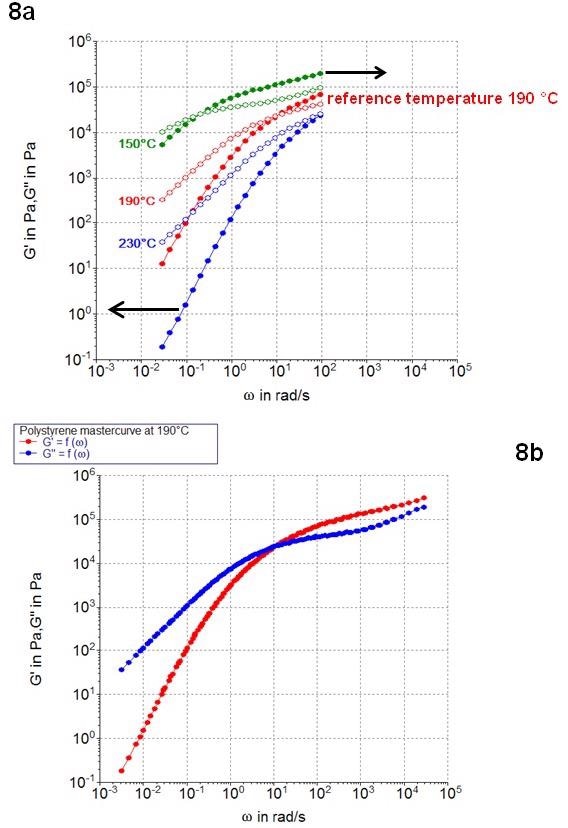
Figure 8. Application of the Time-Temperature-Superposition principle with a polystyrene melt. Image Credit: Thermo Fisher Scientific – Materials & Structural Analysis
It is possible to divide the master curve into three regions. At low frequencies, the sample is in the terminal region prompting the polymer melt to exhibit predominantly viscous behavior.
Material behavior in the terminal region is controlled by long molecule chain relaxation processes, while G’ and G’’ typically have slopes of 2 and 1 in a double logarithmic plot in this region.
At medium frequencies, however, a transition takes place with a crossover between G’ and G’’. In this scenario, viscoelastic behavior is primarily driven by the polymer’s molecular weight distribution.
At the highest frequencies, the sample exhibits predominantly elastic behavior, with G’ larger than G’’. In this scenario, the polymer’s behavior is controlled by the rapid relaxation motion of the shortest polymer chains.
G’ and G’’ data obtained over a wide frequency range can also be employed in the calculation of molecular weight and molecular weight distribution for a significant number of linear thermoplastic homopolymers.
This is achieved by ensuring that the tested frequency range includes data from the low frequency terminal region to the end of the high frequency plateau region.
Using Dynamic Mechanical Thermal Analysis to Investigate Final Product Properties
It is also possible to utilize rotational rheometers in Dynamic Mechanical Thermal Analysis (DMTA), applying this technique to solid, rectangular-shaped polymer specimens.
DMTA testing involves a material being exposed to oscillatory mechanical excitation while its temperature is continuously altered.
Data acquired throughout this process can be used to identify characteristic phase transitions, for example, glass transition, melting and/or crystallization within the polymer matrix.
DMTA can also be used to evaluate final product performance and to investigate the robustness of specific application-based properties, such as brittleness, stiffness, damping or impact resistance.
Figure 9 displays an example DMTA test performed on a semi-crystalline polyetheretherketone (PEEK) sample.
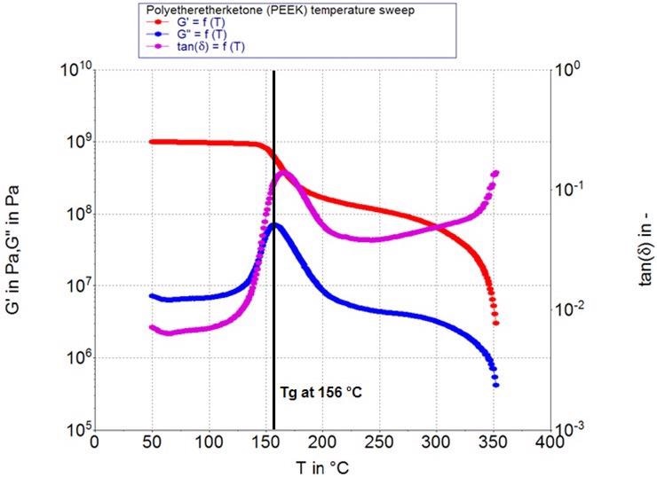
Figure 9. Storage modulus G’, loss modulus G’’ and tanδ as a function of temperature for a polyetheretherketone. Image Credit: Thermo Fisher Scientific – Materials & Structural Analysis
This was tested from below its glass transition to slightly under its melting temperature, supported by the use of a specialized solids clamping tool designed for rotational rheometers.5
A lab scale injection molding system was used to prepare the rectangular sample.6 A material’s glass transition can be identified using different metrics under rheological testing, with the most common metric utilizing the maximum in the loss modulus G’’.
The initial decrease in the storage modulus G’ or the maximum in the tanδ (G’’/G’) can also be used to highlight glass transition.
In the example presented in Figure 9, the maximum in G’’ is found in the center of a wider transition range, while the onset of the G’ decrease is close to the beginning of the transition. The maximum in tanδ is found close to the end of this range.
Figure 10 showcases the generalized behavior of a polymeric sample during a temperature sweep test.
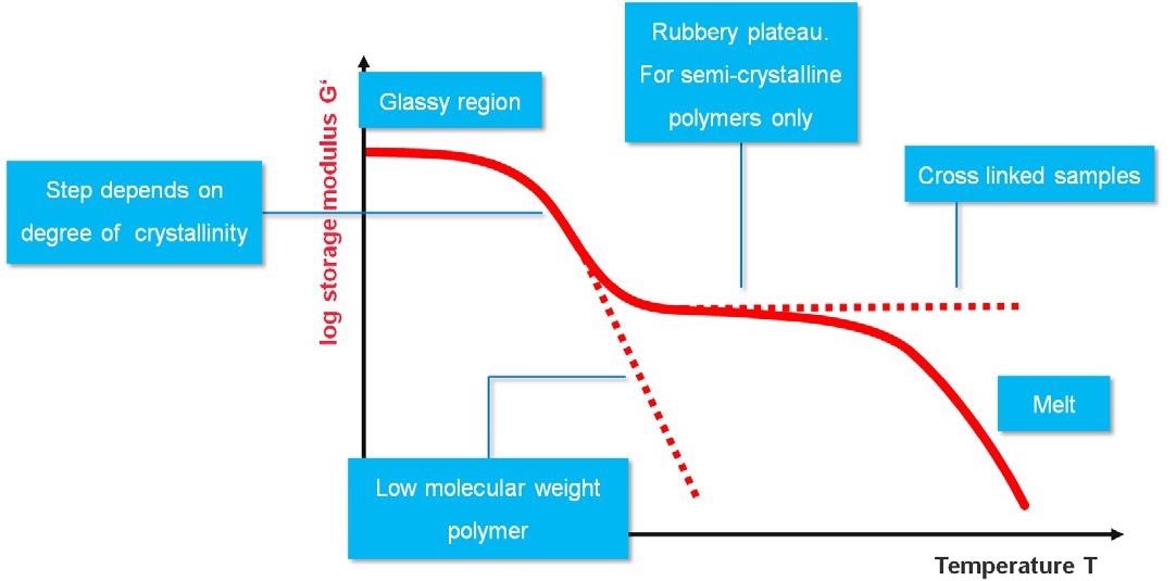
Figure 10. Generalized behavior of polymer sample in a DMTA test. Image Credit: Thermo Fisher Scientific – Materials & Structural Analysis
Semi-crystalline polymers will always transition from a glassy region at low temperatures, shifting to a rubbery plateau and ultimately into their melt state when subjected to higher temperatures.
The step height from the glassy region to the rubbery plateau is dependent on the polymer’s degree of crystallinity - as the degree of crystalline domains in the polymer increases, this, in turn, causes a decrease in step height between the two regions.
It should also be noted that low molecular weight polymers do not exhibit a rubbery plateau. In these examples, once the glass transition is complete, the material will change to a soft melt with G’ decreasing in line with increasing temperature.
Cross-linked polymers do not melt at all, however. These remain in a rubbery state until the onset of thermal decomposition.
Benefits of Extensional Testing
Extension is the third primary flow type that can be investigated rheologically. Extensional flows occur in processes such as spraying and vessel filling, but these are not very common for polymer melts.
Rather, extensional flows tend to occur in polymer melt processes in the form of film blowing, fiber spinning, injection molding or foam extrusion.
Figure 11 illustrates transient extensional viscosity at a range of extensional deformation rates for two different polyethylene samples.
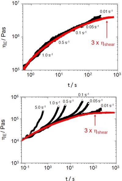
Figure 11. Extensional viscosity as a function of strain rate for a non-branched HDPE (top) and highly branched LDPE (bottom). All tests were performed at 150 °C. Image Credit: Thermo Fisher Scientific – Materials & Structural Analysis
These tests were conducted using the Sentmanant Extensional Rheometer (SER) fixture designed for use with rotational rheometers.7
The plot on the left displays the extensional behavior of a non-branched high-density polyethylene (HDPE) sample - no observable strain hardening occurred for this type of material.
The plot on the right displays the results of identical experiments and was performed with a highly branched low-density polyethylene (LDPE) sample.
The red curves in the images indicate transient shear viscosities multiplied by three according to the Trouton ratio for uniaxial extension.8 This shear viscosity data was acquired via rotational step experiments.
The extensional behavior of the branched LDPE sample was notably different from the behavior observed in shear flow, unlike the linear HDPE sample. The LDPE sample displayed shear hardening behavior throughout extensional testing, particularly at higher deformation rates.
Strain hardening behavior offers advantages to polymer processing techniques, including film blowing or fiber spinning. A comprehensive understanding of a polymeric material’s extensional behavior is a key factor in optimizing its final product properties.
This behavior cannot be measured and evaluated using standard rotational rheological measurements.
Conclusion
Knowledge of a polymeric material’s viscoelastic properties is key to optimizing formulations and blends, adapting a process to accommodate the properties of a specific material, and minimizing the risk of flow anomalies.
The use of rotational rheometers to perform appropriate rheological tests facilitates the investigation of a polymers’ viscoelastic behavior; from the melt-state to the solid-state and all points in between.
Acquired data can be utilized in the optimization of processing conditions and final product performance, as well as for establishing structural property relationships.
Their usefulness and applicability are major drivers in rheological tests’ wide use in the analysis of polymeric fluids, both in industry and academia.
References
- C.W. Macosko, Rheology: Principles, Measurements, and Applications, Wiley-VCH; New York (1994).
- W.P. Cox and E.H. Merz, Journal of Polymer Science, 28, 619 (1958).
- J.D. Ferry, Viscoelastic Properties of Polymers, 3rd ed., John Wiley & Sons, N.Y. (1980).
- J. Dealy, D. Plazek, Time-Temperature Superposition – A Users Guide, Rheology Bulletin, 78(2), (2009).
- C. Küchenmeister-Lehrheuser, K. Oldörp, F. Meyer, Solids clamping tool for Dynamic Mechanical Analysis (DMTA) with HAAKE MARS rheometers, Thermo Fisher Scientific Product Information P004 (2016).
- Thermo Scientific HAAKE MiniJet Pro, Thermo Fisher Scientific Specification Sheet (2014).
- C. Küchenmeister-Lehrheuser, F. Meyer, Sentmanat Extensional Rheometer (SER) for the Thermo Scientific HAAKE MARS, Thermo Fisher Scientific Product Information P019 (2016).
- F. T. Trouton, Proc. R. Soc. A77, 426−440 (1906).
Acknowledgments
Produced from materials originally authored by Fabian Meyer and Nate Crawford from Thermo Scientific.

This information has been sourced, reviewed and adapted from materials provided by Thermo Fisher Scientific – Materials & Structural Analysis.
For more information on this source, please visit Thermo Fisher Scientific – Materials & Structural Analysis.