What is Superconducting Qubit Characterization?

Exploiting quantum physical phenomena, quantum computing promises an advance in numerical processing power over traditional computing^{[1, 2]}. The experimental work being undertaken currently in this field focuses on improving the devices that would ultimately perform the function of transistors in classical processors - the quantum bits (qubits).

One of the most promising contenders studied currently are superconducting qubits^{[3, 4]}. As they are based on purely electrical control and microfabrication technology, superconducting qubits are provided with a clear roadmap for large-scale integration of hundreds of qubits in a single processor.

The steady improvement of coherence times achieved over the last few years inspires confidence that the devices can be engineered to a quality that supports practical numerical algorithms.

Growing Complexity

Complex pulsed microwave signals on multiple channels with accurate synchronization are required to control superconducting qubits. With the increase in the number of channels and qubits, standardized, strongly integrated, and highly reliable electronic control solutions are essential.

This demand is addressed by the Zurich Instruments UHFLI instrument, as it combines an arbitrary waveform generator (AWG) that synthesizes precisely shaped pulsed signals, and a 600 MHz lock-in amplifier equipped with digitizer for detection.

By combining generation and detection in one device, the setup complexity and rack space can be reduced, synchronization can be improved, and advanced control methods can be enabled based on feed-forward from detection to generation, for example, sequence branching.

This article discusses how the UHFLI instrument can be used to characterize superconducting qubits in terms of their coherence time, qubit state lifetime, and frequency. Tuning the pulse shapes that are used to generate quantum computing sequences is also provided by the measurements presented in this article.

The circuit quantum electrodynamics architecture, ^[5] which can be extended to the multi-qubit experiments, was used to perform the experiments discussed in this article. The measurements were performed in Prof. A. Wallraff’s Quantum Device Lab at ETH Zurich, Switzerland.

Setup and Sample

Quantum computing devices are developed to enable control and readout of a qubit’s quantum state. The quantum state is generally a quantum superposition of two physical configurations of the qubit device, which encodes the data processed in a quantum computer.

Figure 1(a) displays a sample consisting of niobium- and aluminum-based resonant circuits on a sapphire chip. The actual qubit is a nonlinear resonator formed of an on-chip capacitor (orange in the image) and a small superconducting quantum interference device (SQUID).

With the SQUID design, the qubit frequency can be tuned over a frequency range between 4 and 7.5 GHz by modifying a small magnetic field applied to the device.

A coplanar waveguide (green) directs external signals directly to the qubit for its control. The qubit is coupled with a coplanar-waveguide resonator (blue)^[5] at 4.78 GHz. An on-chip filter connects the readout resonator to a pair of coaxial cables that provide the interface for reading out the quantum state of the qubit.

Figure 1 (b) shows a schematic of the measurement setup where the sample is installed in a dilution refrigerator to offer a well isolated low-temperature environment protecting the sample’s quantum properties.

Figure 1. (a) Optical micrograph of the sample showing the readout resonator (blue) and the qubit capacitor plates (orange). The resonator is coupled to input and output lines via a Purcell filter ^[6] (cyan). Insets show magnified views of the qubit and the coupler between resonator and Purcell filter. (b) Simplified diagram of the experimental setup based on the UHFLI instrument integrating a lock-in amplifier and an AWG. The superconducting qubit sample is cooled in a dilution refrigerator.

Quadrature modulation of a microwave signal is performed with two AWG channels to generate control pulses. Feeding one of the AWG marker channels to the gate input of a signal generator helps to generate the pulses for qubit readout.

The pulses are amplified after they are transmitted through the readout resonator, and then the readout signal is down-converted to an intermediate frequency f_IF. One of the UHFLI lock-in amplifier channels is then used to measure the pulses.

Measurements

Qubit Spectroscopy

The spectroscopic measurements of the line-width and frequency of the qubit and the readout resonator are measured first. The optimum magnetic field bias is set by using a small coil at the sample, and can also be determined using spectroscopy.

In order to measure the readout resonator, a continuous microwave tone is applied to a resonator and the amplitude of the down-converted transmitted signal is measured with the lock-in amplifier. The tone’s frequency v_res is swept across the frequency f_res of the resonator. Figure 2 (b) shows one such measurement. The resonator’s transmission lineshape is a narrow dip at f_res on top of a broader peak, which is the result of the on-chip Purcell filter ^[6] .

A two-tone microwave technique was used to measure the qubit transition frequency. The first microwave tone is applied at a fixed frequency close to resonance f_res to the readout resonator. A second tone is applied to the qubit gate line and its frequency ν_qb is swept across a broad range while the transmission amplitude is measured.

Due to dispersive coupling between the readout resonator and qubit, there is a change when ν_qb becomes resonant with the qubit transition at f_qb ^[5]. As shown in (a), this results in a feature at f_qb.

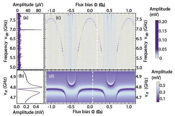
Figure 2. Spectra of the qubit (a) and of the readout resonator (b). The measurement in (a) is obtained by measuring the transmission at a fixed frequency ν_rf close to the cavity resonance (b) and sweeping the qubit drive frequency ν_qb. (c) The arc-shaped dependence on magnetic flux F is characteristic for this type of qubit. As the qubit frequency crosses the frequency of the readout resonator along the horizontal axis in (d), the two exhibit an avoided crossing. The color scale shows the amplitude of the signal transmitted through the readout resonator after amplification.

In Figure 2 (c) and (d), the qubit and resonator spectra can be seen as a function of magnetic field. The qubit transition frequency exhibits a characteristic, arc-shaped dependence on magnetic field ^[7]. As can be seen in (d), an avoided crossing is exhibited by the readout resonator and the qubit. The strong coupling between the resonator and the qubit is the cause of this vacuum Rabi splitting.

In order to probe the qubit’s dynamic properties, the subsequent measurements are pulsed rather than continuous. A pulse sequence that consists of a readout part and a control part form the basis of these measurements. Pulses are applied to the qubit gate line at a frequency close to f_qb during the control part.

These resonant pulses result in Rabi oscillations, a coherent oscillation of the qubit between its ground and excited state. After the control part, a pulse is applied to the readout resonator at a frequency close to f_res, and a trigger measurement of the signal is performed after transmission through the sample.

In order to achieve this, the return signal is first down-converted in the analog domain to f_IF = 28.125 MHz. It is then demodulated in the digital domain with the lock-in amplifier. Using digital lock-in technology instead of direct down-conversion to DC, the measurement is protected from amplifier offset voltage drift and 1/f noise ^[8].

To increase the signal-to-noise ratio and average out quantum fluctuations, the entire cycle is repeated several thousand times. Conventionally, the averaging of raw data is done before the down-conversion. With the UHFLI’s digital demodulators, down-conversion can be performed before the averaging.

This method removes one data post-processing step from the experiment, and it eliminates the requirement of choosing an intermediate frequency that is commensurate with the repetition rate. It is also necessary during the implementation of feed-forward protocols where the demodulated signal must be available quickly.

Rabi Oscillations

Applying a control pulse results in a distinct change of qubit state, which can be used as a single-qubit gate operation. Such operations are necessary for implementing quantum computing algorithms,in a similar way that the logical inversion is required for classical computing algorithms. The pulse parameters for a given gate operation can be determined using a Rabi oscillation measurement.

A control pulse with an envelope shaped by smooth edges (rise/fall time 3.9 ns) and a flat plateau with a variable width are generated for this measurement. Following this control pulse is a readout pulse, which is a microwave burst with an approximately rectangular envelope.

The probability of the qubit being in the excited state follows a sinusoidal evolution as a function of the control pulse area, which is also proportional to its width at half maximum. This evolution is reflected in the signal measured during the readout phase that is plotted in Figure 3.

The curve enables the width of the qubit gate pulses relevant for the next measurements to be identified: the Π -pulse width corresponds to the first maximum, the Π/2-pulse width corresponds to the first quarter period. While the p-pulse brings the qubit from its ground to the excited state, the Π/2-pulse brings the qubit to an equal coherent superposition of ground and excited state. All control pulses were repeated 4000 times at a rate of 13 kHz, for this measurement.

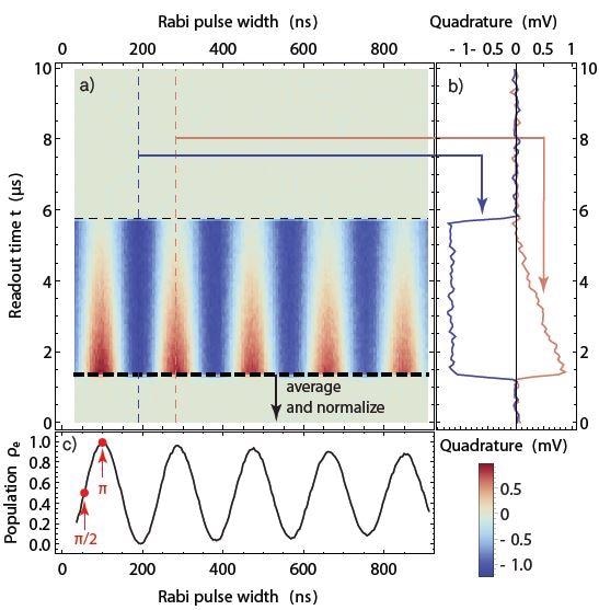
Figure 3. Rabi oscillation measurement. As a function of the width of the control pulse, the qubit evolves periodically from ground state to excited state and back. This results in a sinusoidal readout signal amplitude as a function of the pulse width (horizontal axis) as seen in the color plot in (a). (b) Time-dependent readout signal at two values of the pulse width marked in (a). The time between about 1.2 µs and 5.8 µs corresponds to the readout pulse. (c) Rabi oscillation plot obtained by averaging the data in (a) and normalizing the result to obtain a mean excited-state population. The measurement allows us to determine the parameters for Π- and Π/2-pulses (red marks).

Qubit Lifetime

The duration of a computation algorithm is restricted due to the decay from the excited qubit state to the ground state. Measurement of the average lifetime T₁ is therefore an important part of the device characterization.

When measuring the T₁, a Π-pulse is applied at the beginning of the sequence, then there is a wait for a variable time t, and the qubit state is finally measured. Figure 4 (a) shows the resulting data. The lifetime T₁ = 8.8 µs is extracted from a fit to an exponential exp(–t/T₁).

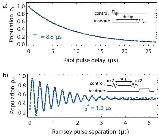
Figure 4. (a) Qubit lifetime T₁ measurement. The qubit is initialized in the excited state with a p-pulse. The subsequent exponential decay is then measured for increasing delays before the readout pulse. (b) Ramsey fringe measurement. As the delay between two p/2-pulses is varied, the qubit readout signal follows a decaying oscillatory evolution reflecting the gradual loss of phase coherence. The measurement is used to determine the qubit coherence time T₂*. Both measurements were averaged 40’000 times at a 27 kHz repetition rate.

Waveforms and sequences can be directly generated using the UHFLI’s control software LabOne^®. A series of 200 patterns were generated with UHF-AWG using a sequencer loop incrementing the readout pulse delay from 0 µs to 26 µs with dynamic waiting times and run-time sequencer variables.

This means that a single Π-pulse envelope that has less than 400 samples of waveform data for both channels can be used to generate all qubit control pulses. This is unlike conventional methods, where patterns for all pulse delays must be uploaded to the AWG sample-by-sample, requiring waveform data of about 200 x (26 µs) x (2 channels) x (1.8 GSa/s) = 18.7 MSa and consequently a much longer waveform transfer time.

Qubit Coherence Time

The free coherent evolution of the qubit is shown by the Ramsey fringe measurement. There are two Π/2-pulses separated by a varying delay time followed by a qubit readout in the Ramsey sequence. When there is no decoherence, the two Π/2-pulses combine to form a full Π-pulse and the qubit ends up in the excited state.

Relaxation and dephasing during the delay time results in the pulse addition becoming imperfect, which means the potential for being in the excited state decays with the delay time. A slight detuning of the pulse frequency relative to f_qb creates a beating effect between the qubit phase and the phase of the control pulse carrier. This leads to an oscillatory contribution in the readout signal. A dephasing time of T₂*=1.2 µs can be extracted from the measurement shown in Figure 4 (b).

The pulses that are generated by the duel-channel AWG have intermediate-frequency carriers at 112.5 MHz, generated using the UHF-AWG modulation mode operating in the digital domain. The intermediate frequency is then upconverted to the qubit transition frequency using an analog mixer. The use of amplitude modulation means that phase and carrier frequency can be adjusted or swept without reprogramming the AWG.

Conclusion

These essential qubit measurements demonstrate the potential of the Zurich Instruments’ UHFLI lock-in amplifier and AWG in an experimental domain requiring timing precision, signal quality, and high speed. An in-depth characterization of a qubit instrument in terms of its lifetime, coherence time, and operating frequency can be obtained from the measurements. More complex sequences for experiments such as randomized benchmarking or spin echo are set up in a straight-forward manner based on the elementary pulses used for these measurements.

Acknowledgements

Zurich Instruments would like to thank Prof. Wallraff and his team for sharing experimental results and for their strong commitment to developing qubit experiments with Zurich Instruments technology. Special thanks go to Michele Collodo for carrying out the measurements and providing an excellent framework for the integration of the UHFLI into the existing laboratory infrastructure. We thank Theodore Walter for providing the qubit sample and Yves Salathe, Simone Gasparinetti, and Philipp Kurpiers for support with the measurements and for discussions. This work was supported by the Swiss Federal Department of Economic Affairs, Education and Research through the Commision for Technology and Innovation (CTI).

References

^[1] R. P. Feynman. Simulating physics with computers. Int. J. of Theor. Phys., 21:467, 1982.

^[2] T. D. Ladd, F. Jelezko, R. Laflamme, Y. Nakamura, C. Monroe, and J. L. O’Brien. Quantum computers. Nature, 464:45, 2010.

^[3] Y. Nakamura, Pashkin, Yu. A., and Tsai J. S. Coherent control of macroscopic quantum states in a single- Cooper-pair box. Nature, 398:786, 1999.

^[4] John Clarke and Frank K. Wilhelm. Superconducting quantum bits. Nature, 453:1031, 2008.

^[5] A. Wallraff, D. I. Schuster, A. Blais, L. Frunzio, R.- S. Huang, J. Majer, S. Kumar, S. M. Girvin, and R. J. Schoelkopf. Strong coupling of a single photon to a superconducting qubit using circuit quantum electrodynamics. Nature, 431:1627, 2004.

^[6] M. D. Reed, L. DiCarlo, B. R. Johnson, L. Sun, D. I. Schuster, L. Frunzio, and R. J. Schoelkopf. High-fidelity readout in circuit quantum electrodynamics using the Jaynes-Cummings nonlinearity. Phys. Rev. Lett., 105:173601, Oct 2010.

^[7] Jens Koch, Terri M. Yu, Jay Gambetta, A. A. Houck, D. I. Schuster, J. Majer, Alexandre Blais, M. H. Devoret, S. M. Girvin, and R. J. Schoelkopf. Chargeinsensitive qubit design derived from the Cooper pair box. Phys. Rev. A, 76:042319, Oct 2007.

^[8] David Schuster. Circuit Quantum Electrodynamics. PhD thesis, Yale University, 2007.

This information has been sourced, reviewed and adapted from materials provided by Zurich Instruments.

For more information on this source, please visit Zurich Instruments.