To extract the maximum information from any sensor, system calibration and data processing corrections play a crucial role for making precise measurements. Instrument limitations frequently present themselves as noise effects in the returned signal, distorting or masking information that is present. This can severely limit a given instruments sensitivity, dynamic range, accuracy and resolution. The type scale of calibrations corrections needed vary based on to the device being used. Most array based sensing instrument will need some form of flat field correction process applied to their output to guarantee a uniform response.
This is predominantly true of spatial heterodyne spectrometers such as the HES range of instruments produced by IS-Instruments Ltd. These instruments comprise of multiple elements that effect the final output, including the detector and internal optics. The HES range are static Fourier transform spectrometers, and thus have a number of similarities with Fourier transform instruments
Several processes which are usually applied to classical FTIR instruments should be part of the data processing for a HES instrument. These include:
- Flat field correction
- Dark noise subtraction
- Phase correction
A complete mathematical description of how to process SHS data can be detected in [2, 3]. Other methods can also be applied to the data in order to enhance the signal to noise ratio (SNR) or accuracy in signal reconstruction such as:
- Apodization
- Smoothing or filtering
- Zero filling
- Ghost fringe removal
Besides these common data processing tools, FT based devices have also successfully used the so called super gain techniques such as Maximum entropy in order to extract more information.
Of the techniques described above, the most noteworthy is the application of the flat field correction. This article describes its application to HES data and the corresponding effect on the collected spectral information. It demonstrates the gains that can be made by careful application of this process.
Flat Field Correction Principle – Raw Data
The purpose of flat field correction is to remove variations in instrument/detector sensitivity on a pixel-to-pixel basis. The flat field is attained by examining a so-called flat image. This could be a calibrated white light frame in a dispersive spectrometer.
The observed variations from the expected calibrated frame are produced by instrument variations. If this image is attained with a sufficient SNR, it can then be used to divide in subsequent data to “flatten” the response. In a dispersive system, this effect is usually dominated by differences in the detector sensitivity. In modern scientific grade CCDs, this difference is typically less than 1%. Thus, these effects are usually localized and effortlessly removed in a dispersive spectrometer.
A FFT is applied to the imaged frame to extract the spectra in a HES instrument. Consider using a near perfect HES instrument where all pixels, with the exception of one, have similar quantum efficiency when measuring a perfect monochromatic source. In this case, the image obtained would be a perfect sine wave, with only one outlying pixel shown with the red oval (LHS in Figure 1). After Fourier Transforming this data, the sine wave would be transformed into a single peak at one particular frequency, however the outlying pixel would convert into a sine wave of a given amplitude and frequency, effecting a major fraction of the acquired spectrum (RHS in Figure 1). This sine could mask other spectral information present in data. Thus, it is extremely essential to take every single step in order to remove any of these variations or discontinuities. This can result in a single pixel having a vital influence on the observed spectra response as illustrated in Figure 1.
(It should be noted that the figure is not to scale and the actual amplitudes of the two functions are proportional to their relative energy within the discrete step and the sine).

Figure 1. Effects of non-flat response in a HES instrument.
Procedure
Flat Field Correction of HES Spectrometer:
In addition to detector differences generating a non flat response in a HES, it is possible for environmental effects to influence the image observed. For instance, localized dust on one of the lenses could affect the transmission of collected light through a portion of the instrument. Thus, it could be essential to take the flat field frame once every 2-3 months. An additional complication with a HES is that the interference fringes developed by the spectrometer must be removed from the flat fielding process. Therefore, the flat frame is independently attained from each grating.
The technique gathers dark image and non-interferometric grating images, from each diffraction grating. This information is then used to produce a flat field image which can be applied to the raw image data of a measured sample. The data is corrected using the equation:

Where IR is the raw image, D is the dark frame, and F is the acquired flat frame. A sample of potassium nitrate (KNO3) was measured in order to demonstrate the process of flat field correction on actual data
The instrument used was an ISI HES2000 coupled to a F2:1# probe with the sample analyzed in a backscatter configuration. The data was full vertically binned to guarantee high levels of SNR.
Flat Field Correction Method:
The method used to collect, process, and apply flat field data to the raw image files is described in Table 1.
Table 1. Process of flat fielding the HES data
| Data collection and dark frame subtraction |
| 1. |
Collect multiple raw image frames |
100 frames used |
| 2. |
Sum images and compute the average frame |
|
| 3. |
Collect dark image |
100 frames used |
| 4. |
Sum dark images, compute the average frame and subtract from the image gathered in step 2 |
|
| Acquire flat field |
| 5. |
Cover lateral grating |
|
| 6. |
Acquire images from a broad band source |
100 frames used |
| 7. |
Cover axial grating |
|
| 8. |
Acquire images from a broad band source |
100 frames used |
| 9. |
Compute the average flat frame for each grating and subtract the average dark image |
|
| 10. |
Sum the results from both gratings and normalize the data |
i.e. so that the mean value is 1 |
| Application of the flat field |
| 11. |
Remove the profile shape from the flat field frame |
|
| 12. |
Divide the data from step 4 by the flat frame from step 11 |
|
| 13. |
Compute the power spectrum |
|
Measurement and Application
Flat Field Measurement
Figure 2 displays the image frame obtained from the KNO3 sample using the HES spectrometer, the data was attained with a 0.2 second integration time. The image has been apodized using a Hanning window. The Gaussian profile produced by the fiber illumination must be noted. The strong center burst is positioned at 1000 pixels, and this indicates that the spectrum acquired has a vital broadband component. Figure 3 shows the Raman spectrum of the KNO3 sample extracted from Figure 2. The data is displayed in the pixel space. Two peaks are visible at approx. 280 and 410.
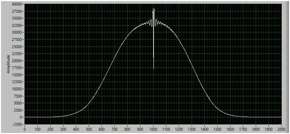
Figure 2. FVB apodized interferometric image of Potassium Nitrate using 1mm fibre coupled HES and F2 backscatter probe
Additionally, there are two notable points of interest:
- The spectra display a vital background signal with a steady baseline raising towards the LHS (this is because of sample fluorescence)
- The spectral baseline is extremely noisy, which potentially masks smaller peaks that may be present.
No increase in the integration time or averaging could bring down the apparent noise in the data, indicating that a basic or instrument limitation was being observed.

Figure 3. FFT of image shown in Figure 2, gives Raman spectra of KNO3
Figure 4 shows the flat field image acquired by merging separately captured data from each grating. The interference pattern is removed as expected, but also the underlying Gaussian profile has changed.

Figure 4. White: Full 2000 pixel wide flat field image formed of merged data from each diffraction grating and Red: polynomial fitted curve
This shape differs every time the fiber is removed and reinserted into the instrument, due to minute changes in its physical location with respect to the spectrometer. It is vital that this shape is removed from the flat field frame before it can be applied to any data. Otherwise this difference dominates the final response of the instrument.
Figure 5 displays this data from pixels 850 – 1120 in order to observe structure present on the image. This highlights a huge distortion between pixels 970 and 975, together with other artifacts along the curve.
The red line in Figure 5 is a fitted curve that will be employed to remove the profile shape observed in the image. This shape is produced by the fiber input.

Figure 5. White: central pixels between 850 and 1120 from full flat field image shown in Figure 4 formed of merged data from each diffraction grating and Red: polynomial fit of curve
Effect of Flat Field on Image
Figure 6 displays the calculated flat field once the profile shape has been removed. In this instance, the fiber profile was computed by segmenting the profile shown in Figure 4 into 20 portions and applying a high order polynomial to each. Some structure related to non-ideal curve fitting is observed at 0-100 and 1900-2000. However, the effect of this structure is negligible once the data has been apodized.

Figure 6. Calculated flat field using measured flat field images and multiple order polynomial curve fit
Figure 7 (a) – (c) shows the result of the application of the flat field correction to the apodized image. The effect in the image plane, appears to be relatively modest.

Figure 7. Comparison of uncorrected and corrected images at regions (a) full 2000 pixels (b) central 800 to 1200 pixels only and (c) pixels 900 to 990: white is the raw data; red is the flattened data
Effect of Flat Fielding on Spectra
The importance of this result is completely appreciated when the FFT is applied to the flat field corrected image. This result is displayed in the below figures (red) and differs from the uncorrected spectra (also shown in the below figures (white)).
The baseline noise is majorly reduced throughout. An estimate of the apparent signal enhancement can be computed by comparing the peak at 410 pixels to the standard deviation measured between 900 – 970 pixels. This establishes the fact that the SNR has improved by a factor 1.6. Additionally, the data now displays an additional small peak or cluster of peaks present at approximately 530 pixels.

Figure 8. Flat field corrected (red) and uncorrected (white) Raman spectra of KNO3. Corrected spectra offset for easy viewing.

Figure 9. Central region (from x=250-600) of flat field corrected (red) and uncorrected (white) Raman spectra of KNO3. Corrected spectra offset for viewing.
It is now possible to confirm that this peak has been successfully brought out of the noise floor by comparison of the spectra to a ‘stock’ spectra (Figure 8) in the appendix.
Figure 8 shows 4 distinct peaks 1x ~700 cm-1, 1x ~1050 cm-1 and 2x 1350 cm-1. The uncorrected HES spectra successfully identify the high intensity central and LHS peaks, but the lower intensity RHS doublet peaks are not detectable above the noise floor of the baseline. The RHS doublet peaks are detected, after the application of the flat field correction to the data, demonstrating the importance and strength of the correction procedure in order to identify weaker Raman scattering centers.
Conclusions
This article has described a procedure for flat field correction in spectral heterodyne spectrometers. This has been attained by collecting flat field data from the instrument followed by the computation of a flat field frame. This flat field frame has then been applied to sample raw image data. Major enhancement in the spectral information obtained following conversion of the corrected raw image frame into the power spectrum was observed.
The application of the flat field correction to the raw frame data collected from a KNO3 demonstration sample pointed out the advantages this process yields in successfully identifying weak Raman scatterers. It is now possible to readily and routinely apply this correction procedure to raw image data gathered from any sample measured using the ISI HES Raman spectrometer.
References
[1] https://en.wikipedia.org/wiki/Flat-field_correction
[2] Harlander. J., R. J. Reynolds and F. L. Roesler, “Spatial Heterodyne spectroscopy for the Exploration of Diffuse Interstellar Emission Lines at Far Ultraviolet wavelengths” Astrophys. Journal.Vol. 396, pp 730-740. 1992
[3] Englert. C. R., J. M. Harlander, J. G. Cardon and F .L. Roesler “Correction of Phase Distortion in Spatial Heterodyne Spectroscopy” Applied Optics 43 2004

This information has been sourced, reviewed and adapted from materials provided by IS-Instruments, Ltd.
For more information on this source, please visit IS-Instruments, Ltd.