Different Sieving Methods for Varying Applications

The solidity of concrete, the taste of chocolate, or the solubility of drugs – these are just a few examples of chemical or physical material properties which are affected by particle size. Thus, the knowledge and determination of the particle size distribution plays a major role in the quality control process for industrial products. From research and development to incoming and production control, sieve analyses are used to simply determine the particle size or several parameters. High accuracy, low investment cost, and ease of handling make sieve analysis a commonly used procedure for determining the particle size. This article gives an overview of the various sieving techniques and explains the necessary steps needed to ensure reliable results.

Sieving is performed to separate a sample based on its particle sizes by submitting it to mechanical force. The chosen sieving method determines the intensity, direction, and type of force. The sample is moved either in vertical or horizontal direction. Both movements are superimposed in tap sieve shakers. Air jet sieving is a unique case, where the sample is dispersed by an air jet blown out of a rotating nozzle.

Which Factors Need to be Established to Select a Suitable Sieving Method?

Particle Size

Classical dry sieving is the preferred method when the required measuring range lies between roughly 40 microns and 125 mm. As shown in Figure 1, the range may be extended to 10 microns by air jet sieving and to 20 microns by wet sieving.

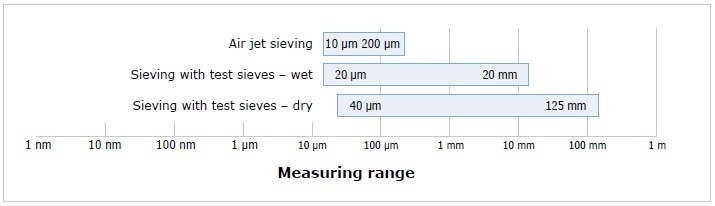
Figure 1. Measuring range of air jet, wet and dry sieving

Sample Properties

Certain factors should be taken into consideration like whether the particles form agglomerates, the type of density of the material or if it is likely to be electrostatically charged.

Standards

The DIN standard 66165 describes the various sieving techniques. If industry-specific standards or test procedures exist, these will also determine the method of choice.

Number of Fractions

Are several fractions needed? Or is it enough to know which percentage of the sample is bigger or smaller than a defined particle size? The process of acquiring the latter information is known as a sieve cut because the sample is merely separated into two fractions.

Different Sieving Methods

After these questions are adequately answered, one can then choose an appropriate sieving method. This article describes the different sieving methods.

Vibrational sieving (Figure 2): In vibrational sieving, the sample is submitted to three dimensional movements. A circular movement superimposes a vertical throwing motion. This mechanism causes the particles to be uniformly distributed across the entire sieving surface and to be thrown into the air where they ideally change their orientation in a way that enables them to be compared to the sieve apertures in all probable dimensions.

Vibratory sieve shakers such as the AS 300 control, AS 450 basic and control, and the AS 200 series (Figure 3) are based on this principle. All RETSCH vibratory sieve shakers may be used for both dry and wet sieving. In addition, the “control” models can be calibrated and allow software-based assessment of the sieving process. They also provide reproducible and globally comparable results due to sieving with controlled acceleration, which is described below.

Sieving with controlled acceleration: The Sieve Shakers, such as AS 450 control, AS 300 control, and AS 200 control, are activated in their natural frequency. In other words, the sieving frequency changes with the load of the instrument. It depends on the sample quantity and the weight of the sieve stack. To ensure the reproducibility of the results even in short-time sieving procedures, the default setting of the vibration height can be switched to sieve acceleration (sieving with equal acceleration). The RETSCH Sieve Shakers — AS 450 control, AS 300 control, and AS 200 control — are the only sieve shakers that have the potential to eliminate influences of error by varying sieving frequencies through automatic amplitude adjustment.

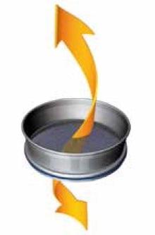
Figure 2. Principle of vibratory sieving

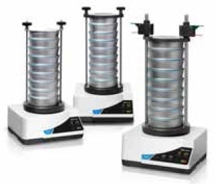
Figure 3. Vibratory sieve shakers of the AS 200 series

Table 1. A suitable vibratory sieve shaker for every requirement

	AS 200 basic	AS 200 digit cA	AS 200 control	AS 300 control	AS 450 basic	AS 450 control
Measuring range	20 µm - 25 mm			20 µm - 40 mm	25 µm - 125 mm	25 µm - 125 mm
Sieve diameter	100 / 150 / 200 / 203 (8") mm			100 / 150 / 200 / 203 (8") / 305 (12") / 315 mm	400 / 450 mm	400 / 450 mm
Amplitude in mm	1 – 100%	0.2 – 3.0	0.2 – 3.0	0.2 - 2.2	0.2 - 2	0 – 2.2
Maximum load	3 kg			6 kg	15 kg	25 kg
Recalibration and sieve acceleration	-	-	yes	Yes	-	yes

 

Wet sieving: Wet sieving is a special case of vibratory sieving. The sieving process may be complicated by electrostatic charging, agglomeration, or a high degree of fineness of the sample. In such cases wet sieving may be required. In this process, the sample is washed through the sieve stack in a suitable medium which is generally water.

Horizontal sieving (Figure 4): This method subjects the sample to a circular horizontal movement. However, the particles do not change their original orientation by this two-dimensional motion. Horizontal sieving is mostly suitable for longish, fibrous or disk-shaped samples (sieving with circular motion according to DIN 53 477). For this type of application, RETSCH provides the AS 400 control that comes with an electronically controlled speed of 50 to 300 rpm. Sieve diameters of 100 mm / 150 mm / 200 mm / 203 mm (8") / 305 (12") mm / 315 mm / 400 mm can be used to separate bulk samples of up to 15 kg in a single run. 45 µm to 63 mm is the measuring range. RETSCH’s EasySieve^® evaluation software can be used to recalibrate and control the horizontal sieve shaker.

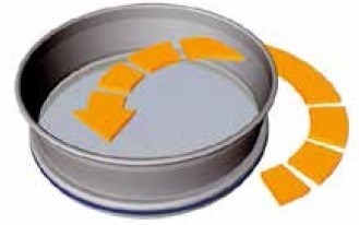
Figure 4. Principle of horizontal sieving

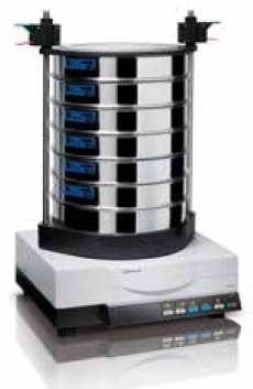
Figure 5. Horizontal sieve shaker AS 400 control

Tap sieving (Figure 6): Several standards stipulate the use of tap sieve shakers. In the tap sieving process, a vertical tapping motion superimposes a circular horizontal movement as, for instance, in the AS 200 tap (speed 280 rpm, taps 150 per minute). The AS 200 tap, shown in Figure 7, can accept up to 7 sieves with diameters of 203 mm (8”) or 200 mm and a maximum sample load of 3 kg. The same evaluation software EasySieve^® can be used to control this sieve shaker.

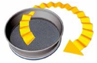
Figure 6. Principle of tap sieving

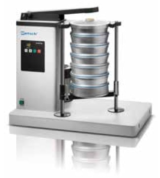
Figure 7. Tap sieve shaker AS 200 tap

Air jet sieving (Figure 8): In order to achieve a sieve cut by air jet sieving, only a single sieve is used rather than a stack of sieves, and the sieve itself is not put into motion. Low pressure inside the sieve chamber is generated by an industrial vacuum cleaner and the sucked-in air escapes with high speed from the rotating slit nozzle placed below the sieve and disperses the particles which can be subsequently compared to the sieve apertures.

As soon as the particles hit the sieve lid, they are redirected and also deagglomerated. Very small particles are then transported through the sieve mesh and get sucked in. These particles can be collected in a cyclone. The AS 200 jet for air jet sieving (Figure 9), provided by RETSCH, include features like innovative Open Mesh Function to lower the number of near-mesh particles as well as automatic vacuum regulation (accessory). Sieve diameters of 203 mm (8”) and 200 mm can be used with the AS 200 jet, which covers a measuring range between 10 µm and 4 mm. EasySieve® evaluation software can be used to control the machine.

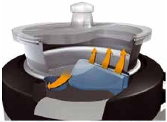
Figure 8. Principle of air jet sieving

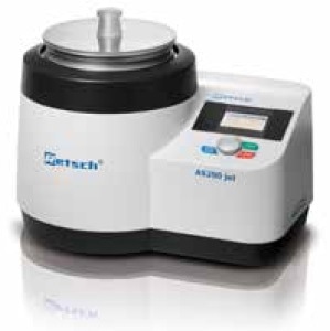
Figure 9. Air jet sieving machine AS 200 jet

Sieve Analysis Step by Step

A complete sieving process includes the following steps which should be performed in a precise careful manner.

a) Sampling
b) Sample division (if required)
c) Selection of suitable test sieves
d) Selection of sieving parameters
e) Actual sieve analysis
f) Recovery of sample material
g) Data evaluation
h) Cleaning and drying the test sieves

Sampling

To achieve a representative lab sample, correct sampling is very important particularly if the material is heterogeneous. Some key questions should be clarified beforehand:

• Which quantity is needed to ensure representativeness of the original sample?
• From which part of the original material should the sample be taken?

Directions and guidelines on the correct sampling process are provided by some industry-specific standards, for instance DIN 51701 in the coal industry. It contains, for instance, the formula

    G [kg] = 0.07 [kg/mm] x z [mm]

which specifies the amount of sample “G” to be extracted from a bulk sample with maximum particle size “z” to achieve a representative quantity. Tasking a coal sample with a maximum particle size of 5 cm as a case in point, the following calculation applies:

    G [kg] = 0.07 kg/mm x 50 mm
     G = 3.5 kg

As a result, the amount of the extracted sample should be a minimum of 3.5 kg to ensure it is representative. For materials other than coal, a different density should be considered.

Sample Division

When the amount of sample is too large for analysis, it must be divided in a way that the part sample represents the original material. Sampling can be performed either manually or randomly by coning and quartering, but these methods are prone to errors and may cause standard deviations that amount to 10% and more just by imprecise division (Figure 10, C + D).

RETSCH’s automated sample dividers like the PT 100 (Figure 11) or PT 200 provide a much more precise and easy method. In the PT 100 rotating sample divider, the sample flows via a feed hopper directly into the openings of a dividing head. Even if there is a coarse-grained sample, the deviations among the amounts collected in each sample vessel are negligible. The division process runs entirely automatically. The dividing head – which can feature 6, 8 or 10 outlets – produces a controlled constant 11 rotations per minute, irrespective of power and load frequency. This means when a dividing head with 10 outlets is used, the sample flow is divided almost 1100 times per minute. Therefore, the highest possible degree of division accuracy is statistically ensured.

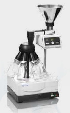
Figure 10. Rotating sample divider PT 100

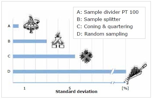
Figure 11. Standard deviations of analysis results resulting from different sampling methods

Selection of Suitable Test Sieves

Sieve selection not only depends on the sample quantity but also on the approximate particle size distribution. The increments of the mesh apertures should follow a logarithmic series to cover the complete particle size range of the sample. This is usually performed with the aid of the Renard series, for instance R10/3. The standard DIN 66165 includes guidelines on the selection of mesh sizes and sieve diameters. It also specifies the maximum sample load allowed for different mesh sizes and the maximum particle size (Figure 12).

Mesh size	Max. batch	Max. permitted sieve oversize
25 µm	14 cm3	7 cm3
45 µm	20 cm3	10 cm3
63 µm	26 cm3	13 cm3
125 µm	38 cm3	19 cm3
250 µm	58 cm3	29 cm3
500 µm	88 cm3	44 cm3
1 mm	126 cm3	63 cm3
2 mm	220 cm3	110 cm3
4 mm	346 cm3	173 cm3
8 mm	566 cm3	283 cm3

Figure 12. Examples for the maximum batch and permitted sieve oversize for 200 mm sieves (according to DIN 66165)

Calculation of sieve load: The oversize on a sieve with a 1 mm mesh size, for instance, should not be more than 20 cm³ per square decimeter. For a sieve of 200 mm, that equals 63 cm³ oversize and for a sieve of 400 mm it is 252 cm³. However, the maximum batch should not be more than twice the amount of the oversize value, that is, a 200 mm sieve with a mesh size of 1 mm should not be filled with more than 126 cm³ sample material. When these values are multiplied with the bulk density, the corresponding masses can be achieved.

The maximum sieve oversize allowed on a sieve can be roughly calculated with the formula

    R = 0.00178 x D² x w^0.667 x ρ

where R stands for the maximum permitted sieve oversize in [g]; w is the mesh size in [mm]; D represents the sieve diameter (200 mm / 300 mm etc.), and ρ describes the material density. In the above example and in the standard 66165, a density of 1 kg/dm³ was assumed. The standard 66165 also describes the maximum load per sieve which should never go beyond the maximum sieve oversize D by more than twice the amount.

The maximum particle size allowed can be calculated by using this formula

     x_max = 10 x w^0.7

where x_max [mm] is the maximum particle size allowed, and w stands for the nominal mesh size of each sieve (the value is used in the formula without unit). For a sample on a sieve with a 250 µm-aperture size, the following calculation is used to establish the maximum particle size allowed:

    x_max = 10 x w^0.7
     x_max = 10 x 0.250^0.7
     x_max = 3.79 (unit = mm)

Selecting Suitable Sieving Parameters

Company-specific regulations or industry-specific standards usually contain data about the required sieving parameters. If this is not the case, then those parameters would have to be established by experiment. The sieving time and also the amplitude, when using vibratory sieve shakers, are the most critical factors. Observing the maximum sieve load can protect the sieve against damage and ensure that every particle has the potential to compare with the sieve mesh as often as possible and in every dimension.

Amplitude

During any sieving process, there is a constant size comparison between particles and sieve apertures. A particle will pass the mesh if it is smaller than an aperture and when it does not pass the aperture it is thrown upwards with subsequent lifting of the sieve bottom, takes a different orientation – which is vital with longish particles – and hits the mesh again for a new comparison. Each comparison presents an opportunity for the particle to pass the sieve mesh. Therefore, the aim of a sieving process is to create as many comparisons as possible in a given time. This is preferably the case when within the duration of a sieve bottom vibration, exactly one comparison occurs and the particles which do not pass the sieve mesh are accelerated in a way that within the next duration another comparison occurs. This state is referred to as statistical resonance (blue curve in Figure 13).

If a particle is hardly accelerated or not at all, it will not orientate freely for a new comparison (red curve) and if a particle is accelerated too strongly it will have very few opportunities to compare with the sieve apertures (yellow curve) and the complete separation of the sample will be delayed.

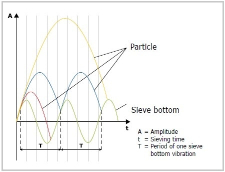
Figure 13. Movement of particles in avibratory sieve shaker in relation to the sieve bottom

Blue curve: The particle is in statistical resonance with the sieve bottom; red curve: the particle is not adequately moved; yellow curve: the particle is thrown too high

The set amplitude decides the acceleration rate of a particle. The optimum amplitude for a specific material and quantity should be established empirically. Here, amplitude means the complete oscillation in the horizontal plane, both above and below the idle position. A 1.2-mm amplitude indicates a movement of + 0.6 mm and – 0.6 mm relative to the idle position.

Sieving Time

According to the DIN 66165 standard, the sieving process is assumed to be completed when, after one minute of sieving, feed quantity of less than 0.1% passes the sieve. The sieving time should be extended if the undersize is larger. Experience has shown that vibratory sieving in three dimensions is mainly suitable for acquiring a sharp separation of fractions in a short period of time.

Carrying Out the Actual Sieve Analysis

The actual sieving process begins only after the selection of parameters. The following steps should be performed in chronological order:

1. Put together a sieve stack with collecting pan.
2. Choose sieving aids, if needed: for mesh sizes measuring less than 500 microns, the use of brushes, cubes, or chains is advised to ease the passage of sample.
3. Establish the empty weight of the collecting pan and sieves: This can be done manually or software-based by using a balance. Appropriate programs such as EasySieve^® make weighing and evaluation processes much easier.
4. Place the sieve stack with growing mesh size on the collecting pan (Figure 14)
5. Weigh the sample and place it on the top sieve (biggest mesh size); fasten the sieve stack on the machine
6. Set the speed / amplitude and sieving time on the sieve shaker
7. Begin the sieve shaker
8. After the sieving time has ended, weigh each sieve and the collecting pan with the fraction on it
9. Determine the percentage and mass of each fraction
10. Evaluation

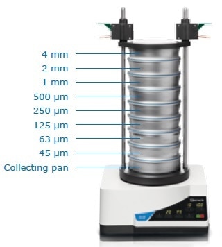
Figure 14. Stacking of sieves (example)

Recovery of Sample

The material is removed from the sieves once the sieving process is completed. Fraction recovery is an important advantage of sieve analysis when compared to most optical measurement techniques. In addition to being analytical values, the fractions also physically exist and can be used for additional processes after sieve analysis.

Determination and Evaluation of Data

Determination and evaluation of data evaluation can be done either manually or with the help of the EasySieve^® software. As listed in Table 2, the percentages are measured and shown graphically (Figure 15).

Table 2. Example of a sieve analysis

Sieve [µm]	Net weight [g]	Weight after sieving [g]	Difference [g]	Percentage p3 [%]	Cumulative distribution Q3 [%]
Pan	501	505.5	4.5	3	3
45	253	259	6	4	7
63	268	283	15	10	17
125	298	328	30	20	37
250	325	373	48	32	69
500	362	384.5	22.5	15	84
1,000	386	401	15	10	94
2,000	406	412	6	4	98
4,000	425	428	3	2	100
			= 150 g	= 100%

 

The empty sieves are weighed both before and, containing the respective fractions, after the sieving process and the difference corresponds to the weight of each fraction. When these are put into relation to the total sample weight, the percentage of each fraction can then be measured. The advantage of this method is that owing to the absence of dimensions, sieving is performed independently of the mass or density of the sample material. Sieve loss refers to the difference between the sum of the single fractions and the weighed sample. If this is more than 1% of the feed quantity the sieve analysis must be repeated according to the DIN 66165 standard. The fractions’ mass percentages can be graphically shown as histograms (Figure 15). In the example used here, the largest fractions can be found between 250 microns and 500 microns with 32%.

The cumulative distribution curve Q₃ is achieved (Figure 16) by adding up the single fractions and through interpolation between the measuring points. This curve helps to establish a wide range of sample properties. Taking a look, for instance, at the particle size of 250 microns the corresponding value of 36% can be read off the y-axis which means that 36% of the total sample is smaller than 250 microns, as shown in Figure 17. Further, the corresponding particle size (330 microns) is read off the x-axis to find out the median Q₃ (50) of this distribution. This means that 50% of the sample mass is equal or smaller than 330 microns. In this fashion, different Q₃(x) or x(Q₃) values can be established. The EasySieve^® software enables fast and error-free assessment of various parameters.

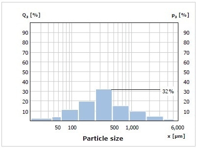
Figure 15. Histogram with percentages of the fractions

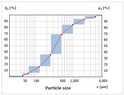
Figure 16. Histogram with cumulative distribution curve of the fractions

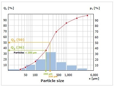
Figure 17. Cumulative distribution curve with exemplary percentages

Cleaning and Drying of Test Sieves

Test sieves are actually measuring instruments which must be treated with care before, during, and after the sieving process. During the sieving process, the sample should never be forced via the sieve mesh during the sieving process. Even a mild brushing of the material – especially through very fine fabric – may change the mesh and damage the sieve wire gauze. Near-mesh particles may get trapped in the sieve mesh and these can be removed by simply turning the sieve upside down and tapping it lightly on a table. For particles that cannot be removed this way, a fine hair brush can be used to lightly brush the underside of the sieve mesh.

Using a hand brush with plastic bristles, coarser fabrics with mesh sizes greater than 500 microns can be effectively cleaned wet or dry. Sieves with less than 500-µm mesh size should be cleaned in an ultrasonic bath. Different sizes of drying cabinets can be used for drying test sieves which should be placed vertically within the cabinet. It is advised not to exceed a temperature of 80 °C. At higher temperatures, the fine metal wire mesh could become warped and therefore, the tension of the fabric within the sieve frame is reduced but this makes the sieve less efficient.

The Fluid Bed Dryer TG 200 from RETSCH is mainly effective in drying test sieves with a diameter of 200 or 203 mm. The plastic or rubber seal rings should be removed before drying or cleaning the sieves. If there are deviations from the uniformity of the mesh, it means the sieve is not suitable for quality control purposes (DIN ISO 9000 ff) and hence needs to be substituted

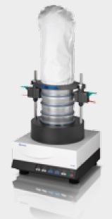
Figure 18. Fluid Bed Dryer TG 200

Conclusion

For particle size analysis of bulk materials, sieve analysis continues to be a well-established method and is described in various standards. Sieve analysis offers exact and reproducible results while being easy to perform and maintaining the physical size fractions. Investment costs are also much lower when compared to, for instance, optical measurement systems. The various sieving methods are fully covered by RETSCH’s offering which includes the ideal sieve shaker for almost any bulk material. RETSCH sieve shakers ensure accurate and reproducible results in the shortest period of time and meet all test agent monitoring requirements according to DIN EN ISO 9000 ff.

This information has been sourced, reviewed and adapted from materials provided by RETSCH GmbH.

For more information on this source, please visit RETSCH GmbH.