Thermo Scientific™ X-ray Photoelectron Spectrometers are fitted with a microfocusing monochromator, as well as a multi-channel detector. This combination of features makes them well suited for chemical state mapping.
The maps’ spatial resolution is defined by the X-ray spot size selected by the user. The multi-channel detector enables snapshot spectra to be collected at every pixel of the map; an approach that is significantly quicker than scanned acquisition.
These spectrometers feature a charge compensation system that allows chemical state maps to be created from insulating materials with ease.
Sample Preparation
A copper grid was fixed to a substrate made up of silicon coated with an acrylic acid plasma polymer. Next, the substrate was placed in a plasma that contained a fluorocarbon monomer. This resulted in the fluorocarbon polymerizing on the parts of the substrate that were exposed to the plasma.
Following exposure to the plasma, the grid was separated from the substrate, leaving behind a patterned, polymeric fluorocarbon. Figure 1 shows the preparation method as well as the area of the sample which was analyzed in the Thermo Scientific™ K-Alpha™ XPS system.
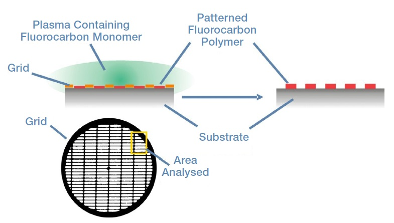
Figure 1. An illustration of the sample preparation, the grid used in the preparation, and the area of the sample analyzed in K-Alpha.
Analysis Conditions
Here, the monochromated X-ray spot size was set at 30 µm. Snapshot XPS spectra of C 1s and F 1s were collected into 64 channels for each individual element. This set of spectra was acquired at each pixel in an array of 67 x 94 pixels at a 10 µm step size. This was achieved by scanning the sample stage.
Peak Fitting Spectrum
Figure 2 displays the C 1s spectrum which was determined by summing the C 1s signal from the entirety of the image. This spectrum clearly illustrates the presence of both ester and fluorocarbon species.
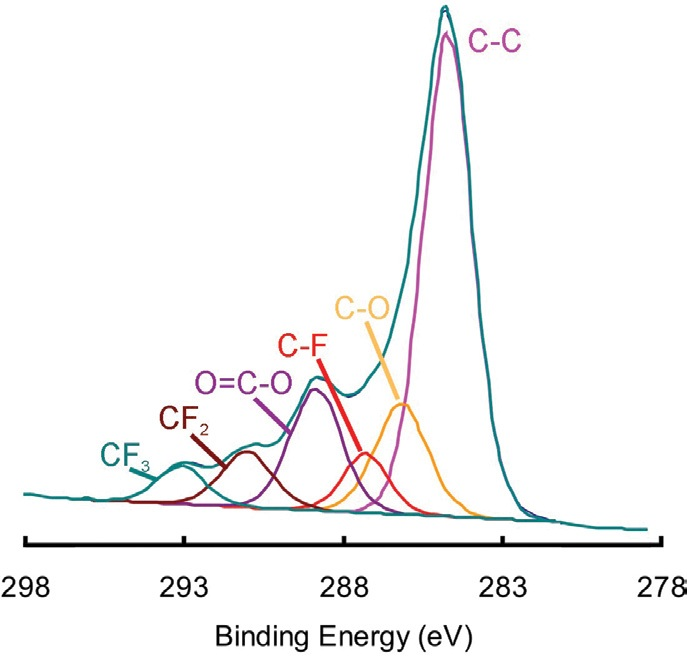
Figure 2. Peak fitting of the C 1s spectrum obtained by summing the spectra in each of the pixels of the map.
Image Construction
One simple means by which a map can be generated is that of displaying the image produced at a specific binding energy. Figure 3 displays images formed at 10 of the 64 binding energies collected for this measurement.
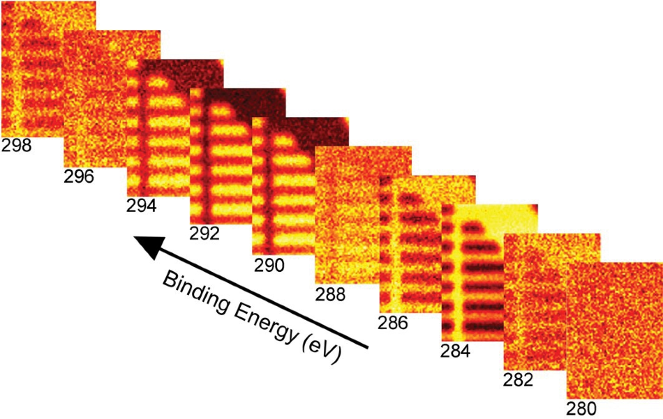
Figure 3. Maps constructed at 10 of the 64 binding energies collected.
Figure 4a displays an image created from binding energy of 284.7 eV (hydrocarbon), while Figure 4b displays an image of the peak at a binding energy of 291 eV (a fluorocarbon peak). Figure 4c is an overlay of both these images.
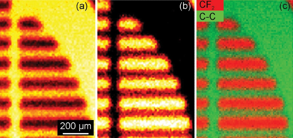
Figure 4. (a) Map obtained from the signal at a binding energy of 284.7 eV (the hydrocarbon peak) (b) Map obtained from the signal at a binding energy of 291 eV (a fluorocarbon peak) and (c) an overlay of the maps shown in (a) and (b).
Having completed the peak fit (Figure 2), it is possible to fit each of the spectra that constitute the map with the same set of peaks. This allows images to be created from any of the fitted peaks displaying fitted peak areas or atomic concentration.
For example, Figure 5 illustrates atomic concentration images, and in this example, non-linear least-squares fitting was utilized with the data set to create atomic concentration maps for both components.
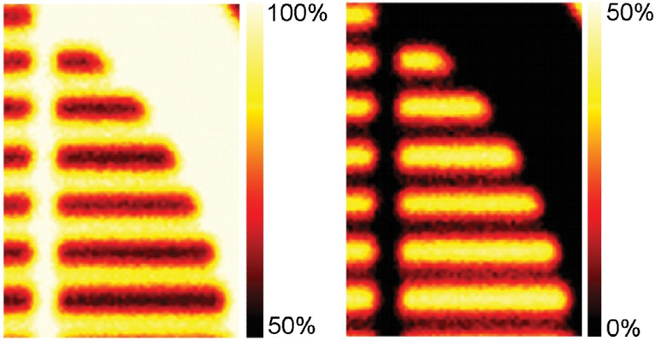
Figure 5. (a) Atomic concentration map from the hydrocarbon peak following peak fitting at every pixel. (b) Atomic concentration map from the fluorocarbon peak.
Reconstructed Spectra
Each individual pixel in the image contains a spectrum, meaning it is possible to sum the spectra from specified areas on the image to produce a small area spectrum. Figure 6 displays two spectra created from the image’s indicated parts.
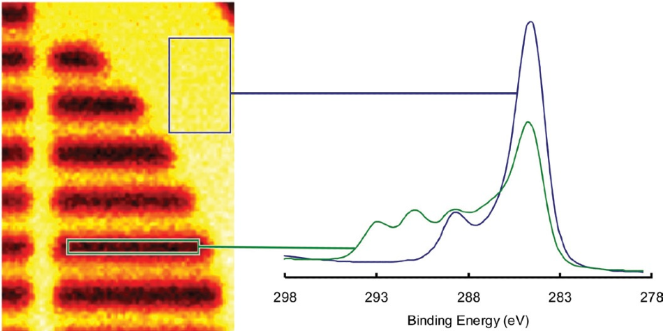
Figure 6. C 1s spectra reconstructed from the areas indicated on the map.
It is clear in this example that the substrate peaks may be seen in the fluorocarbon region, while no fluorocarbon can be seen in the substrate region.
Thickness Map
In the areas of the sample covered by the fluorocarbon material, peaks can be detected from the substrate. This implies that the fluorocarbon layer is just a few nanometers thick.
It is possible to build a thickness map of the sample using the ‘Overlayer Thickness Calculator’ - a fundamental component of the Avantage data system. The only assumption made in this particular calculation was that the density of each individual polymer was equal to its bulk density. Figure 7 displays the measurement results.
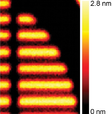
Figure 7. Thickness map of the fluorocarbon layer.
Advantages of Stage Scanning
The K-Alpha spectrometer’s sample stage is scanned to produce a map, and this means of map acquisition offers a series of advantages over other approaches:
- Spatial resolution is defined only by the X-ray spot size, which is constant throughout the whole acquisition. This means that there is no image quality degradation at the edges.
- Having a spectrum at each pixel allows quantitative maps of chemical states and thickness maps to be easily constructed.
- The spatial resolution is not affected by the settings of the transfer lens, meaning that the spectrometer is always used at its maximum transmission.
- The point on the sample being mapped is consistently at the optimum analysis position, meaning there can be no differences in sensitivity across the field of view.
- X-ray energy and intensity are not affected by the position of the sample.
- A huge field of view is possible - up to 60 x 60 mm for K-Alpha.
Conclusions
The K-Alpha XPS system is able to produce high-quality images. Parallel acquisition of spectral information (snapshot spectra) ensures that acquisition is quick and the considerable number of channels collected in each individual spectrum allows quantitative, chemical state mapping to be performed reliably.
Cutting-edge features available in the Avantage data system deliver clear chemical state information, illustrating the way in which chemical states are distributed in two dimensions. In cases where there is a thin overlayer present (such as this example), it is feasible to measure and map the thickness of that overlayer in a non-destructive way.
Acknowledgments
Thermo Fisher Scientific would like to thank Kristina Parry and Jason Whittle of Plasso Technology Ltd., UK for supplying the sample analyzed in this work.

This information has been sourced, reviewed and adapted from materials provided by Thermo Fisher Scientific – X-Ray Photoelectron Spectroscopy (XPS).
For more information on this source, please visit Thermo Fisher Scientific – X-Ray Photoelectron Spectroscopy (XPS).