Three tools are typically used to measure vibrational noise (noise) - a storage Oscilloscope (scope); a vibration sensor (sensor), which is generally a 'seismic grade' accelerometer1; and a two-channel spectrum analyzer with sub-Hertz capability (analyzer).
The scope is used to observe the sensor's signal in the time domain, and the analyzer can perform Fourier analysis on the sensor's signal to provide a frequency domain picture of the same data.
Although this looks simple, a scope can only indicate the peak level of the noise but cannot provide the root-mean-squared (RMS) value or the 'frequency of the noise.' What is the meaning of a 'peak' value? Is it a sensible question to ask what the 'frequency' of noise is? What is the meaning of an RMS value? Generally, it is not correct to ask what the 'frequency of noise' is. Likewise, an RMS value does not have any meaning unless a frequency range over which it is calculated is specified.
Similarly, an analyzer calculates amplitude spectrum or amplitude spectral density. One is expressed in Volts and the other in V/√Hz ("Volts per root Hertz"). Which should be used? Most analyzers default to the amplitude spectrum, which is not the correct way to characterize most noise sources. As a consequence, several users collect meaningless data as the analyzer settings are wrong.
In order to use these tools correctly, it is essential to get a better understanding of the measurable parameter: noise. Noise is characterized as random or coherent2. These can be further divided into stationary or non-stationary. These are different noise sources and need to be analyzed using different techniques. The individual conducting the measurement or survey has to find out the type of noise and measure it appropriately.
Types of Noise: Random vs. Coherent:
How the different types noise look in a scope is shown in Figure 1. The examples were selected to enable easy identification of the different types of noise.
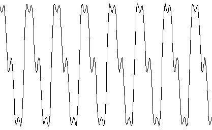
A: Purely periodic (coherent) noise
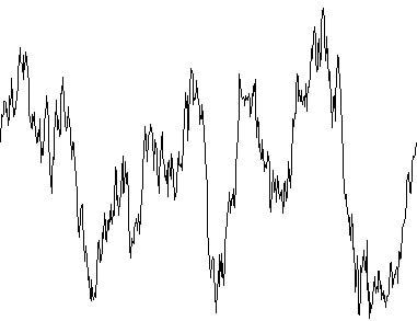
B: Purely random noise
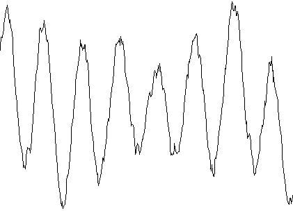
C: Periodic and random noise together
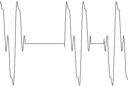
D: Non-stationary periodic noise
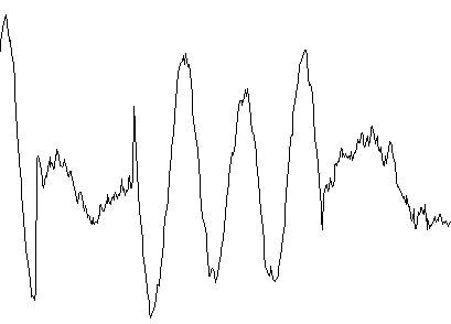
E: Random plus non-stationary periodic noise
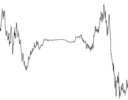
F: Non-stationary random noise.
Figure 1
Curves 1A and 1B show what many people would recognize as noise; but they are the least likely to be observed in the real world. Curve 1C illustrates the most common type of noise: a combination of A and B.
Here, for ease of illustration, the coherent noise source (periodic noise) is shown to dominate over the random noise. However, random noise can also dominate. Frequently, an analyzer has to 'see' the coherent noise in a signal, since the noise component is not usually evident from a scope trace.
In reality, noise almost never has a constant amplitude, but varies with time, and such a noise is known as non-stationary. Curve 1D shows a periodic noise source when randomly turned off and on. Noise produced in a building with an air compressor or HVAC system cycling on and off is shown in curve 1E.
Here, a background of random noise exists, with a periodic component that comes and goes. Other than meaning 'on' and 'off', non-stationary noise can also mean that noise is gradually built or reduced. Curve 1F illustrates non-stationary random noise. Such a noise is common when a microphone is held near a highway, or in seismic noise data when a storm comes and goes3.
Measuring Noise
Scopes can quickly indicate the type of dominating noise during a measurement, and can determine the peak noise level (unlike analyzers). However, these are not used widely, and a spectrum analyzer is the most important tool for quantification of noise. Things can get problematic here.
The simplest noise source to understand and measure is the stationary coherent noise source. As shown in the curve 1A, the signal consists of a pure sine wave, in addition to some higher harmonics (2 ƒ0, 3 ƒ0, 4 ƒ0 and so on). Every signal component has a definite amplitude and frequency.
A spectrum analyzer digitizes this signal, performs a Fast Fourier Transform (FFT) on the digitized data, and provides an amplitude spectrum which shows the relationship of amplitude of the components (in microns or volts) versus the frequency.
In addition to plotting, the frequency and height of every peak can also be tabulated. This method is appropriate to measure the strength of coherent noise sources, even when random noise exists.
Random noise needs another approach as it is fundamentally different. For random noise, there is no longer a specific level or amplitude of signal "at" a particular frequency. In fact, noise does not exist "at" any given frequency. Instead, random noise must be considered in terms of density.
In the volume of air in a room, a lot of air molecules are present but no air molecules exist at a single point. To define the number of air molecules, it is necessary to know the air density and a finite air volume. No volume means air does not exist. It is perfectly legitimate to discuss the average air density at a given point, and that air density is different at various points (air is denser at an individual's feet than at the head). This holds true for random noise also.
For random noise, the equivalent density is known as the amplitude spectral density (ASD) at a specific frequency, and the equivalent volume is referred to as the frequency bandwidth. The number of air molecules is analogous to RMS level of the signal. This, in the context of this article, is the RMS ground motion. The RMS amplitude is expressed as:
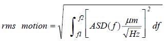
Here, the ASD(ƒ) is a function of frequency, and has units4 of microns/√Hz. The form of the integral shows why the ASD is expressed "per-root-Hertz": this cancels the units of dƒ, and provides the RMS result in the proper units (microns). An analyzer can display the ASD(ƒ) if 1/√Hz or "per-root-Hz" units are chosen.
Just as the number of molecules of air is defined only for a fixed volume, similarly the RMS motion is defined only for a fixed range of frequencies, in this instance, from ƒ1 to ƒ2. The 1/3 octave plot is commonly used to express RMS motions. Here, the frequency spectrum is divided into 1/3 octave5 bins (from 1 to 1.23 Hz, 1.23 to 1.59 Hz, 1.59 to 2.0 Hz and so on).
The integral is performed over each frequency range, after which the resulting RMS values (in microns) are plotted in a bar graph with respect to frequency. In several analyzers, this task is accomplished as a built-in function. To calculate the RMS motion over a wider range of frequency, the quadrature sum6 of all the bins in the range is taken.
In a spectrum analyzer, amplitude spectral density units of [Volts or units]/√Hz must be selected for the vertical scale4, failing which random noise cannot be measured properly. Similarly, if the analyzer is configured to measure a spectral density, it is not possible to measure the correct value of the amplitude for coherent noise sources (in 1/3 octave or ASD formats). The analyzer must be told before whether it is to measure a density or an amplitude.
What the Analyzer Does
Figure 2 shows how coherent and random noise sources behave differently.
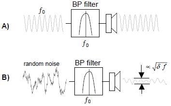
Figure 2
A simple band-pass filter centered on ƒ0 with a width δƒ is linked to a speaker. The bandpass (peak) gain of the filter is 1. Figure 2A shows a sine wave of frequency ƒ0 being applied to the input. The speaker output is the full amplitude of the input, and is not dependent on the width of the filter δƒ.
This is because the filter only eliminates input components away from ƒ0 (and there are none). In contrast to Figure 2A, Figure 2B illustrates the dramatic effect on random noise. The filter gets rid of the energy above the frequency ƒ0 + ½ δƒ and below ƒ0 – ½ δƒ, leaving a signal that sounds closer to a pure tone at ƒ0 when the width of the filter δƒ is narrowed. Additionally, as the filter is narrowed, it blocks more energy, and the output amplitude is reduced in proportion to √δƒ.
A spectrum analyzer is basically identical to a series of band-pass filters similar to that shown in Figure 2, but in the place of speakers, the analyzer measures the amplitude of the filter output(s), and displays the numerical results in graphical form.
It can be shown that the width δƒ of the filters in Hz is about 1/T, where T denotes the duration of the analyzer's measurement and is measured in seconds. In FFT analyzers, the 'filters' δƒ are spaced apart in order to give a full coverage of the frequency spectrum. For instance, a 10 s measurement would provide a 0.1 Hz frequency resolution (filter widths) to result in 100 data points between 1 and 10 Hz.
Figure 2 shows what an analyzer, configured to measure an amplitude spectrum, would see: each and every filter truly transmits the amplitude of any coherent noise at the filter's center frequency. The output amplitudes are plotted by the analyzer, post-measurements. The measurement time T alters the filter widths δƒ, which does not influence the result (as in Figure 2A).
It quickly becomes evident that the filters of Figure 2 generate a nonsensical result for random noise: the noise spectrum amplitude changes as the measurement time T changes. If the measurement is longer, the less noise is observed. Therefore, the random noise level does not depend on how long it is observed.
In order to correct this effect, if the analyzer is configured to measure an amplitude spectral density, it multiplies7 the filter outputs by √T. As T is expressed in 1/Hz, the resulting plot has units of Volts (or microns) per-root-Hertz. Whenever the measurement time T is changed, this factor corrects for the filter bandwidths, and shows a consistent level of spectral density.
Conclusion
Obviously, a factor of √T can be significant, but importantly, amplitude densities and amplitudes are different from each other as are the number of air molecules from gas density. They are not comparable. An exhaustive site survey must follow the steps given below:
1) The analyzer needs to be configured for a 1 - 100 Hertz8 measurement of the amplitude spectrum. All sharp 'spikes' in the spectrum need to be located, and their frequencies and heights tabulated. These would correspond to single-frequency noise sources (compressors, building fans, transformer hum, etc.). The peaks need to be associated with the particular noise sources whenever possible (by turning off the possible sources, and seeing which of the spikes disappear or undergoes changes).
2) The vertical units need to be changed to √Hz. Many analyzers change the amplitude spectrum to an ASD spectrum without recollection of data. After the results are plotted, the results are observed where it can be noted that the heights of the spikes from step 1) have been altered. It is easy for the spikes to be labeled on the ASD plot with their (micron or Volt) values as measured in step 1). The 'background' noise floor close to the spikes correctly denotes the noise density for random noise sources (seismic noise, wind noise, people walking). A single (annotated) plot is obtained that accurately illustrates the noise in an environment.
3) An additional plot can be obtained, if the analyzer can calculate 1/3 octave plots from the ASD. However, the 1/3 octave 'bins' at the spike frequencies can appear as 'spike bins'. The values measured in step 1) on these bins should be observed, if coherent noise sources dominate the noise at those frequencies. If not, the RMS values for those bins can be incorrect by a factor of √T.
4) Any noise sources that might be non-stationary should be noted. Most of these sources would be coherent noise sources: fans, compressors, HVAC systems. As the 'worst case' scenario is usually of great interest, care needs to be taken during measuring of noise when all noise sources are present. Random noise can be influenced by local road traffic, or weather (literally). As it can vary over longer time periods (hours to days), the conditions that can affect ASD measurements should be taken into account.
The person carrying out the measurements needs to determine the types of noise sources that exist, and to collect suitable data. Sometimes, even following the above-mentioned simple steps can be complicated by non-stationary sources. Confusion about the existing vibrational noise issues in a particular environment can be reduced with proper awareness and by carefully noting the possible noise sources.
References
1 Any accelerometer with a sensitivity of 10 V/g or greater, such as the Wilcoxon 731A or PCB 393B12/31.
2 There are also pseudo-random noise sources, like a periodic source which is randomly turned on and off. These are beyond the scope of this article.
3 Wind and coastal waves are major contributors to seismic noise.
4 Analyzers can be configured to convert your sensor's output (in Volts) to an 'engineering unit' like microns or 'g's. Power Spectrums can also be used to measure noise, but these have units of [Volts or units] 2/Hz.
5 An octave is a factor of 2 in frequency. 1/3 of an octave is a factor of 1.23.
6 A "quadrature sum" is the square-root of the sum of the squares.
7 Other correction factors apply due to windowing of the data (Hanning, Brickman, Flat Top, etc.). A discussion of windowing is beyond the context of this article. See Hewlett Packard Application Note 243: "The Fundamentals of Signal Analysis".
8 Common sensors (footnote 1) are poor at measuring noise below 1 Hz, and noise above 100 Hz is usually acoustic in origin – not seismic.

This information has been sourced, reviewed and adapted from materials provided by TMC.
For more information on this source, please visit TMC.