It has never been more challenging to select a particle size analyzer. There are multiple methods from which to select and differences across each method. Sales literature statements about specification and performance are increasingly exaggerated, making it difficult for a first-time buyer. This has resulted in a hindrance rather than a help to the selection process.
A lot of particle sizing instruments were initially created to tackle certain issues. Despite some having discovered additional uses, there is still some truth to the view that some methods are more well-suited for certain tasks. The assertion that one instrument can be appropriate for every particle sizing need and solve all problems is not backed in practice.
Limited in Scope
This article will not explicitly address imaging issues, shape analysis, single particle counting, or sizing of airborne particles. Examples are taken from particle sizing in liquids where the level of material is not of central concern; the ‘dirty water’ or micro contamination issue is eliminated.
This article is a short outline founded on many years of experience with the modern techniques of particle size analysis; it is not conclusive. New methods and new applications of old techniques are frequently appearing. However, the concepts shown here are broad enough to be of value for many years to come.
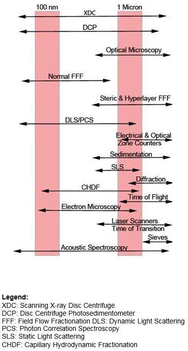
Figure 1. Commercially Available Particle Sizing Techniques (Mostly Liquid Suspensions). Image Credit: Brookhaven Instrument Corporation
Classifications
Particle sizing methods can be categorized in numerous ways.
Size Range: A lot of noteworthy applications in particle size analysis center around 1 micron. Figure 1 displays many commercially accessible methods for particle sizing with a purposefully ‘fuzzy’ demarcation around 1 micron.
What is the reason for the importance of the region around 1 micron?
This region is the general dividing line between sedimentation and centrifugation. For dense and/or large particles, sedimentation is good. For particles that less dense and/or smaller, centrifugation is beneficial. Both density and size have a role; the selection of method varies on both properties.
Second, this region is the general separating line between Fraunhoffer Diffraction (FD) and light scattering. For bigger particles, the classical FD method is separate from the refractive index of the particle. For smaller particles, the scattering pattern varies significantly on the refractive index of the particle.
Third, measurements become more difficult with zone counting (ZC: electro- and photo- zone) methods beneath this region. Electrozone methods are subject to signal-to-noise issues and photozone methods and optical scanners are subject to impacts from diffraction. ZC methods suffer from a rising number of coincidence errors at these smaller sizes.
Fourth, the capacity to resolve images with an optical microscope grows more challenging under approximately one micron.
Each of these statements is a generalization. However, they offer good, first order estimates of the practical working limits of any one method. In some instances, these limits may be surpassed. But size range claims without qualification should be received with caution
Imaging vs. Non-imaging: Instruments built on imaging are, possibly, able to record shape, structure and texture as well as concentration and size. They can preferably differentiate between various compositions. Imaging methods comprise of optical and electron microscopy, video, holography and photography. Image analyzers are frequently, but incorrectly, considered the primary technique of particle size analysis.
Image analysis has many drawbacks and issues. Usually, not enough particles are measured to give consistent statistical outcomes. Manual image evaluation is subjective, slow and labor intensive. As with additional single particle counters, image analyzers may be subject to coincidence effects. When automated and computerized, it becomes increasingly expensive and coincidence impacts may be more challenging to recognize.
Non-imaging methods produce comparable spherical diameters (ESD). This is the diameter of a sphere that would offer the same outcome as the actual particle. Thus, various methods might result in different equivalent spherical diameters for the same particle. These variations are important: They show information on the shape, structure, or texture of the particle. Despite this, if conclusive information of this kind is necessary, then an image analyzer is required.
Degree of Separation: A further key classification is the degree to which particles are divided before measurement. There are three classifications here: single particle counting, fractionation, both limited and high resolution and ensemble averaging.
Single particle counters (SPCs) consist of image analyzers, electro- and photozone counters and particle scanners. Like image analyzers, SPCs are subject to coincidence counting effects. The zone counters are additionally subject to blockage of the zone. Electrozone counters normally need high salt intensities to work properly and this may result in aggregation. However, SPCs are the favored selection when particles need to be counted as well as sized.
Fractionation methods consist of sieving, sedimentation, centrifugation and numerous types of particle chromatography. Subject to how the measurement is taken, the particles might be somewhat split or entirely split. The difference is critical when high resolution outcomes are necessary. As a class, the fractionation methods are fairly slow.
Ensemble averages consist of Fraunhofer Diffraction (FD) and every type of light scattering. The signal, from which the size distribution information is determined is a sum across all the signals from every particle throughout the whole measurement. Therefore, the outcomes are an average across a group of particles. As a class, ensemble averagers are rapid, simple to automate and can be put online. In general, however, the resolution is bad.
Weighting: A size distribution has two coordinates. The size, which is most frequently, an equivalent spherical diameter, is mapped on the x-axis; and the total in every size class, which is mapped on the y-axis. The amount is generally provided as either the amount or volume, or mass of particles. If the particle density is equal for every size, then the volume and mass descriptions are equivalent.
Every particle sizing method weights the amount observed to varying degrees. For instance, light scattering on very small particles is weighted by the strength of scattered light, which fluctuates as the 6th power of the diameter. A few large particles can overshadow the scattered light signal concealing the presence of small particles. Electro zone methods weight by the volume of the particle, which differs as the cube of the diameter.
Despite the simplicity of writing the equations for converting from one kind of weighting to another, the outcomes worked out this way are frequently in error. It is possible that some particles were not measured at all. It is also possible that the measured distribution is considerably broader than the real distribution.
Or, in hybrid methods, different ranges are weighted in varying ways. In each of these cases, the errors in the transformed data are a lot more exaggerated because of weighting.
Whenever feasible, a particle sizing technique that offers the preferred weighting with no transformation. If absolute counts are necessary, then a single particle counter would be preferable. If mass is important, then an instrument responsive to mass would be preferable. If a small number of particles in the tail of the distribution are critical, then an instrument that has the capacity to detect these would be preferable.
Information Content: The final major classification consists of the amount of information necessary to answer a specific problem in particle sizing.
Often just a single number is necessary to resolve a question in particle sizing. That number may be the average size, or it may be a collective requirement like 90% of the particles are under a specified size. For quality assurance or process control, this single number may be adequate. Methods that offer just a single number consist of the following: a turbidity measurement at one wavelength; end-point titration of the surface groups; and the Blaine test for big particles in a powder sample.
Occasionally a second number is necessary. Perhaps it is the width of the distribution (testing for monodispersity) or two cumulative sizes, for example, the 90th and 10th percentile values (portraying the effectiveness of rutile as a pigmenting agent). In the submicron range, DLS is a method that consistently produces a measure of the width in addition to an average of the size distribution.
Further size distribution information is frequently difficult to find and may skew a single, broad distribution, the size and relative numbers of multiple peaks in a multi-peaked distribution, or the presence of a few particles at one extreme of the distribution. Where the distribution has many, closely spaced attributes, a high resolution method is required. More extensive size distribution information is often necessary in the pigment and coatings industry.
Finally, it is pertinent to be cautious. Any of the modern techniques of particle size analysis claim to offer complete size distribution information, although they frequently cannot substantiate this claim. Computers are fantastic devices for storing, retrieving and massaging data; however, apart from image enhancement, computers cannot often improve the resolution in particle sizing applications. That is the role of the standard technique.
Specifying a Particle Sizer
Specifications are of two kinds: quantitative and qualitative. If it is necessary to run 30 samples every day, then you have quantified a throughput specification. One illustration of a qualitative specification is its simplicity to use.
Short lists of both kinds of specifications follow. The lists are not definitive. However, they offer a good starting place for focusing on queries necessary to answer prior to making an informed choice.
Quantitative Specifications
- Reproducibility
- Size Range
- Precision
- Resolution
- Throughput
- Accuracy
Qualitative Specifications
- Life Cycle Cost
- Ease-of-Use
- Support
- Versatility
Size Range: The zero-to-infinity machine is very popular. It seems to resolve lots of issues: just one instrument is necessary, now and for the future; less bench space is necessary; operator learning curves are lessened to one. Its universality is extremely appealing, which has caused zero-to-infinity machines to become extremely popular. This is where hybrid instruments are important; they mix more than one method. However, there are many restrictions with the zero-to-infinity machines. However, the biggest of all is that they do not exist.
First, there are theoretical restrictions with any single method. Diffraction is usually restricted to sizes much bigger than the wavelength of the light source. Sedimentation is restricted at the high end by turbulence (large Reynolds numbers) and at the low end by diffusion. It is not difficult to locate the theoretical restrictions in any method. They lie either in the general assumptions or in the subsequent equations employed to calculate the outcomes.
Second, there are restrictions related to the application of the method in practical instruments. To guarantee a good dynamic signal response, the detectors in diffraction devices are in a way that means the raw size classes are, typically, logarithmically spaced. This could result in the final size class, fully covering half the total size range. Accelerating a centrifuge is useful for speeding up the measurement, but it frequently widens the true size distribution.
Third, there are restricting instances that are wrongly generalized to include all kinds of samples. DLS is a helpful method for particles that stay suspended. Low density materials remain suspended long enough to make valuable measurements, but high-density materials may not. Colloidal gold may be recorded with a centrifuge as low as approximately 0.01 micron due to its high density. Colloidal polystyrene, whose density is extremely small, cannot be measured at much under 0.05 micron employing the same centrifuge. Diffusion causes the outcomes to be questionable and the measurement is extremely slow.
Table 1. Categorizing Particle Size Specifications. Source: Brookhaven Instrument Corporation
| . |
. |
Quantitative
Specification |
Qualitative
Specifications |
| Category I: Academic Use |
|
- Accuracy
- Resolution
|
- Life Cycle Cost
- Versatility
|
| Category II: Research & Development |
|
- Precision
- Resolution
|
- Versatility
- Support
- Cost
|
| Category III: Quality Assurance |
|
- Throughput
- Reproducibility
|
- Ease of Use
- Support
- Repair/Maintenance
|
Fourth, there are restrictions when subranges, or varying methods, are linked together. Usually, every subrange needs a shift in something: a lens, an aperture, a speed of rotation, etc. In theory, this is feasible. In reality, it is challenging to link distributions together without creating artifacts. These are frequently believed to be real by novices. Some manufacturers employ smoothing to conceal these artifacts, yet this could then cause a substantial loss of resolution. Different methods employ different weightings and are subject to different theoretical restrictions, particularly at their extremes. Yet, it is at the extremes where they are linked together.
Despite instrument producers frequently purporting that they have the ideal, universally applicable instrument, the ‘zero to infinity’ machine, most are limited, especially at the extremes of the size range.
Throughput: The idea of throughput is most critical to a quality control laboratory where a lot of samples need to be run in one day. Speed of analysis is sometimes a consideration even for one measurement. Process control applications are an instance of this.
Some methods are fairly slow: Image analysis and sedimentation on small, low density particles are just two illustrations. Some techniques are quite quick: most types of light scattering. In some particle sizing applications, throughput is not actually a concern. In others, it is a major factor. The inexperienced user frequently believes that the measurement duration is adequate to classify the general time per sample. This is incorrect. The exact time includes: sampling, sample preparation, measurement, calculation, formatting and printing and clean up. In some instances, warm-up or calibration, or instrument adjustment can also substantially add to the total time per experiment.
Automated instruments may require time-consuming wash/rinse cycles. Occasionally the measurement duration is just a fraction of the actual time per sample.
Accuracy: Accuracy is a measure of how near an experimental value is to the real value. Often, the real value is not recognized. This could be because the particles are not spherical. It could be because no completely accurate measurements have been taken by which to assess the outcomes. In these instances, accuracy is challenging to assess.
Accuracy is dependent on the knowledge of the sample variables (shape, density, refractive index, etc.) and instrument variables (calibration, alignment, temperature). Good precision suggests good sampling and sample preparation methods have been employed. Occasionally accuracy is critical; occasionally, it is not. Materials employed in the coatings industry must be classified accurately. The big particles impact the film constructing capacity of the coating; the medium size particles impact the light scattering attributes and the small particles control the rheology. In quality and process control applications, comparative changes from batch-to-batch are much more vital than accuracy. In these instances, reproducibility is the main requirement.
Relative numbers are satisfactory if they do not need to be contrasted with other methods or absolute requirements. Then accuracy becomes critical.
Accuracy has frequently been identified by the historical employment of an instrument in a specific field. Although not a true definition, its practicality cannot be overlooked. New instrumentation should concur or, at least, associate with the historical outcomes. But if this argument is carried too far, then bad measurements are perpetuated. Many instruments purport accuracy when tested with spherical standards. There are not many reliable standards. However, there are reference materials for examining precision, reproducibility and resolution. While valuable, these are not absolute standards and, as such, should not be confused with them.
Precision: Instrument precision is a gauge of the variance in repeated measurements on the same sample. Precision restricts resolution, reproducibility and accuracy. Precision is a useful criterion by which to evaluate instruments even if the accuracy cannot be concluded. The precision of a measurement might be +/- 1%. However, the complete accuracy may be a lot worse. It is common to have excellent precision but poor accuracy.
Reproducibility: Reproducibility is a gauge of the variance from sample-to-sample or instrument-to-instrument or operator-to-operator, etc. If there is just one instrument and one operator, then queries of reproducibility might not be particularly interesting. But if there are multiple plant operations with multiple users, all following the same manufacturer’s model, then check reproducibility. If it is much worse than the basic precision of any one instrument, then look for the cause of the mistake. Is it preparation differences or variations from one instrument to the other?
Variations in instrument performance are bigger than most new users would imagine. These can take place due to a change in production method, detector response, software, or a mixture of all three.
Resolution: Resolution has two fairly different meanings in particle sizing. The first meaning affects the minimum detectable differences across various runs. It answers the query, ‘Can the differences between two samples be resolved?’ This description is closely associated with the exactness of the measurement.
The second definition affects the minimum evident differences between elements of the size distribution in one go. The simplest instance is the ratio between two peaks in a bimodal distribution. If the lowest ratio is 2-to-1, then the resolution is quite low. If it is 1.1-to-1, then it is quite high. Group averaging instruments, all kinds of light scattering and diffraction, in particular, are medium to low resolution instruments.
Further than a specific point resolution is not determined by the quantity of channels in an SPC, nor by the quantity of reported size classes, nor by the resolution of the output devices (CRT, printer) employed to organize the outcomes. However, a lot of manufacturer’s requirements would purport that resolution is described in one of these ways. Resolution is, basically, a function of the basic signal-to-noise ratio of the instrument. Reporting over the basic resolution is like increasing the noise: additional numbers are achieved, but they have no meaning.
Over one micron, it is a fairly frequent occurrence for ground material to display very broad distributions. In this instance, resolution does not appear important.
If the basic resolution of an instrument not determined, then it is impossible to know if the broad distribution is truly hiding practical and, perhaps, considerable information? Are those long tails real? Low resolution instruments frequently smear out the distribution resulting in unrealistically long tails.
Accuracy, precision, resolution and reproducibility are purposes of the size range. Mistakes are biggest at the extremes. If it is possible, an instrument should not be purchased with an instrument for measurements at the extremes. A frequent error is to check an instrument in its midrange and then continue to use it at one or another of the extremes.
Claims of accuracy, precision, etc., should be met with skepticism if these truly describe just the average size. If it is not evident from the manufacturer's literature, then clarification should be requested. The average of any distribution is least subject to variation. Even instruments with bad resolution and instrument-to-instrument reproducibility may gain outcomes with 1% or 2% precision in the average for any one instrument. Bigger moments, like the measure of width or skewness and the tails of the distribution, are more susceptible to uncertainties. So specific attention should be given to the variance in some of these more sensitive statistics when assessing instrumentation.
Support: Support is characterized here as good technical support. The manufacturer should be acquainted with your problem. They should be able to suggest sample preparation methods. For support following the purchase, the manufacturer should provide ample training, good technical manuals and experts accessible to aid with results interpretation.
The instrument manufacturer should possess a laboratory with additional instruments accessible with which to substantiate the effectiveness of the suggested instrument. Sample preparation methods are frequently critical to gaining good measurements and the manufacturer should steer you in this part of particle sizing. An ongoing program of development by the manufacturer will guarantee to the user that the instrument will not become outdated soon.
Ease-of-Use: The concept ease-of-use is completely subjective. In one threshold, it means automated sample preparation, automated instrument control and automated data analysis and print out are all unattended.
Some manufacturers aim for this beneath the banner of the ‘one button’ instrument.
Other users believe that an instrument is not complete with incomplete data archiving, retrieval and database management system. These goals are not ‘one button.’ They need a rudimentary knowledge of desktop computer operation.
Versatility: Versatility is here characterized as the capability to measure a broad range of samples and sizes in many different sample preparation conditions. For instance, the electrozone method needs a conducting liquid, which is frequently water with an electrolyte (salt) added. For a lot of applications, this condition is not restrictive; for others, it is. Electron microscopes cannot be employed on samples that sublime beneath a vacuum. Some instruments can be used with nearly every liquid; others cannot. Either the method might be restricted, or its implementation by a specific manufacturer might be.
Summary: The combination and importance of quantitative and qualitative requirements employed in making a choice will be determined by intended use.
It might be hazardous to pigeonhole proposed use by putting it into one of the three categories displayed in Table 1. It may also aid in focusing on what factors are most crucial in solving the particle sizing issue.
Most cannot be so easily categorized. An individual’s research could be a different person's quality assurance. However, if a pattern is identified in one of these categories that is appropriate, this should be employed.
Prior to ending this guide, it is pertinent to highlight two elements of particle sizing that have not been mentioned yet-- sampling and sample preparation. It should be mentioned that most of the variation in particle sizing measurements is ultimately trackable to either incorrect sampling or sample planning. Particle size analysis outcomes are just applicable when the samples drawn are typical and the dispersion techniques suitable.
Sampling and sample preparation should occur prior to particle sizing. Because of this, they are often not directly addressed by manufacturers of particle sizing instrumentation. Yet, they are most likely the main sources of error.
Problem areas to think about:
- Unrepresentative samples.
- Big and/or dense particles caught or isolated prior to reaching the sensing zone.
- Inadequately dispersed samples in the submicron range.
When choosing which instrument to buy, it is common to send samples to numerous manufacturers. The biggest issue in comparing results gained this way is in the belief that all the samples were prepared in the same way. It is a frequent failing to presume the initial measurement stated is right. (This is also true when assessing any new particle size result against the historical database.) A more optimal approach is this: Prepare equally representative samples; establish the optimum technique for dispersing the sample; then instruct every manufacturer to disperse the sample in the same way.
Table 2. Common Traps and Pitfalls in Buying Particle Size Instruments. Source: Brookhaven Instrument Corporation
| . |
- Ignoring correct sampling and sample preparation when comparing instruments and techniques.
- Trying to satisfy several different requirements with one instrument.
- Misunderstanding the best use for different techniques.
- Using values that are computed rather than measured.
|
Table 2 lists a few of the more common traps and pitfalls that can lead to an incorrect choice of particle sizing instrument.
A lot has been written about the fundamentals of particle sizing. The bibliography consists of a few references for those interested.
References
- Terry Allen, Particle Size Measurement, 4th edition, Chapman and Hall, 1991.
- Brian Kaye, Direct Characterization of Fine Particles, Wiley-lnterscience, 1981.
- Modem Methods of Particle Size Analysis, H.G. Barth editor, Wiley-lnterscience, 1984.
- Particle Size Distribution: Assessment and Characterization, T. Provder editor, American Chemical Society Symposium Series 332, Washington D.C., 1987.
- Particle Size Analysis 1988, P.J. Lloyd editor, Wiley-lnterscience, 1988.
- Particle Size Analysis, J.D. Stockham and E.G. Fochtman editors, Ann Arbor Science Publishers Inc., Ann Arbor, Michigan, 1977.
- Bruce Weiner, Let There Be Light: Characterizing Physical Properties of Colloids, Nanoparticles, Polymers & Proteins Using Light Scattering, Amazon Digital Services LLC - Kdp Print Us, 2019.

This information has been sourced, reviewed and adapted from materials provided by Brookhaven Instrument Corporation.
For more information on this source, please visit Brookhaven Instrument Corporation.