Sheet steel has been the most commonly used structural material in the automobile industry since the 1920s. Steel is stiff and robust, making it an ideal option for durable chassis and welded parts.
Steel is now employed in an ever-expanding number of applications, including construction (for example, machinery parts and gears), food (for example, cans), and wear-resistant tools (for example, springs, cutting tools and high-strength wire).
Steel has also demonstrated unparalleled value when used in mass production applications when compared to other materials.
Steel offers many clear advantages, but its most notable and problematic downside remains its low corrosion resistance. Rust on new or used vehicles has been an ongoing issue. As recently a the 70s, enhancements in galvanized coating and base metal quality has been required to prevent rust development.
The presence of rust adversely affects steel’s external appearance and mechanical structure, potentially resulting in premature structural failure that compromises vehicle safety.
One initial solution to steel corrosion was to simply increase the thickness of the components, but heavy components are no longer a viable option due to the current focus on energy-efficient and lightweight materials.
A vehicle’s working life largely depends on the corrosion resistance of its body, prompting the automobile industry to put considerable effort into improving hot-dip galvanized or electrogalvanized zinc coatings designed for optimal oxidation resistance.
The electrogalvanized zinc layer is applied in a series of electrolytic cells, while the sheet steel is immersed in an alkaline zinc solution.
This functions as a cathode, meaning that as an electric current passes through the solution, zinc ions are reduced to metallic zinc on the steel surface, resulting in the creation of a dense, uniform protective layer bonded to the steel.
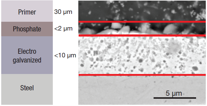
Figure 1. Schematic (left) and SEM image (right) of the different layers. Image Credit: Thermo Fisher Scientific – Electron Microscopy Solutions
A phosphate layer and a primer for the paint are deposited on top of the zinc metal layer (Figure 1), with the zinc phosphate film applied to ensure enhanced base metal protection while improving primer adhesion of the primer. It is porous for this reason.
The standard electro galvanized coating thickness tends to range between 5 µm and 8 µm. It is important to ensure this is as homogenous as possible to ensure good adhesive behavior - both of the coating to the metal and the upper layers to the coating.
The sheet steel surface’s flatness is vitally important if a proper substrate is to be available for high-quality coating. An imperfect or altered rolled steel surface can impact electro-galvanizing and, therefore, adhesion of the zinc phosphate and primer, ultimately resulting in reduced corrosion protection.
This article explores the analysis of a defective coating from a car chassis component – a car door – which had used ultra-low-carbon, titanium-stabilized steel.
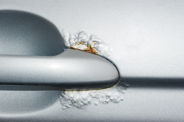
Figure 2. Defective coating on car door. Image Credit: Thermo Fisher Scientific – Electron Microscopy Solutions
The coating was observed to be peeling off (Figure 2), necessitating an understanding of the factors causing the paint to flake and gradually detach from the steel’s surface.
This article presents a rapid, straightforward workflow suitable for identifying the underlying cause of this automotive coating defect and ensuring that any defects are successfully removed prior to the final product reaching customers.
To achieve this goal, it was necessary to characterize the structural and compositional properties via scanning electron microscopy (SEM) and energy dispersive X-ray spectroscopy (EDS).
The Thermo Scientific™ Axia™ ChemiSEM features an integrated, always-on EDS which provides immediate access to an array of compositional data that is central to accurate failure analysis.
Qualitative elemental information is directly linked to the SEM image, enabling considerable time savings and a streamlined workflow.
Analysis
The analysis was initially performed on the surface of a defective part of the sample of interest. Figure 3 (red square) highlights the area where surface characterization was performed.
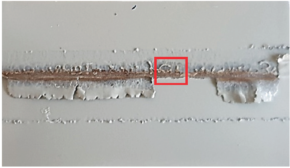
Figure 3. Sample surface. Image Credit: Thermo Fisher Scientific – Electron Microscopy Solutions
Figure 4 shows a low-magnification view of the surface of interest. The grayscale image confirms that this is not protected by any of the coatings. A close-up image was obtained to acquire elemental information and further investigate the morphology of the defects.
One of the primary advantages of the Axia ChemiSEM is its direct link between the EDS signal acquisition and SEM image.
X-rays are collected in the background during a traditional SEM imaging session, allowing these to be shown immediately. Results are available right away – there is no requirement to switch to another software application.
A conventional EDS system would require the operator to re-acquire the image, commence a new EDS data acquisition and post-process the signal to remove the background and address any peak overlaps.
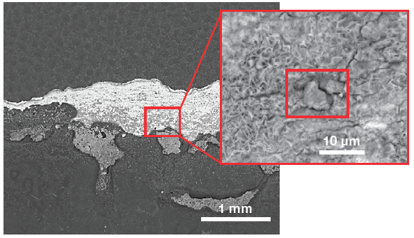
Figure 4. Low-magnification view (left) of the sample surface and a higher magnification of the area of interest (right). (Acc voltage 12 keV, beam current 0.85 nA). Image Credit: Thermo Fisher Scientific – Electron Microscopy Solutions
The spectrum and an array of qualitative elemental information on the area imaged (Figure 4) are displayed via a single click, with both of these highlighting the presence of a foreign particle.
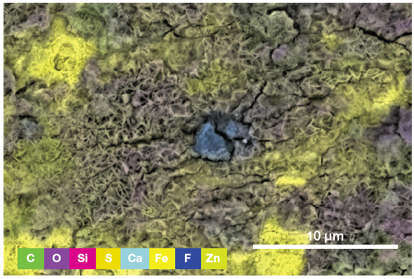
Figure 5. ChemiSEM image showing the involved elements (all activated and shown in this view) and their distribution. (Acc voltage 15 keV, beam current 0.85 nA, acquisition time 60 s). Image Credit: Thermo Fisher Scientific – Electron Microscopy Solutions
To determine the precise nature of the particle, users can select an element to be hidden or shown. This helps provide an improved understanding of the elemental distribution and particle composition.
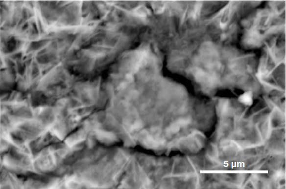
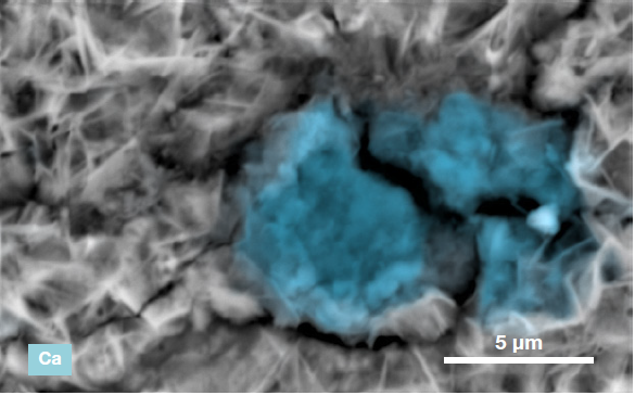
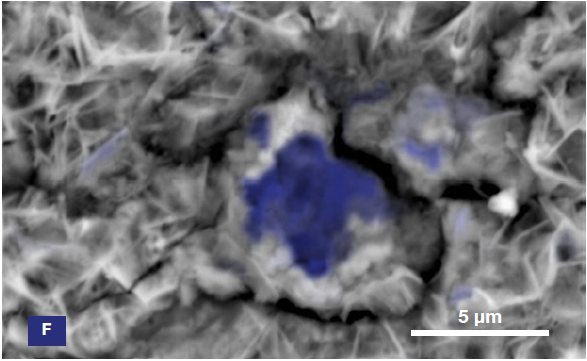
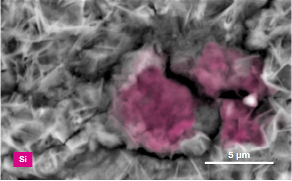
Figure 6. ChemiSEM images of the foreign particle. From top to bottom: backscattered electron image, calcium, fluorine, and silicon distribution. (Acc voltage 15 keV, beam current 0.85 nA, acquisition time 60 s). Image Credit: Thermo Fisher Scientific – Electron Microscopy Solutions
These steps can be performed within the same image acquisition. Qualitative information is provided as the collected signal is post-processed prior to being presented.
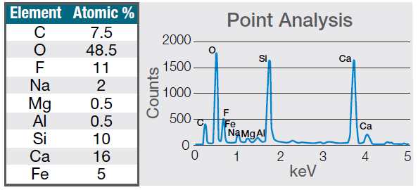
Figure 7. Quantification (left) and spectrum (right) of a 30-seconds area analysis acquired on the defect (Acc voltage 15 keV, beam current 0.44 nA). Image Credit: Thermo Fisher Scientific – Electron Microscopy Solutions
The example particle presented here was found to contain significant amounts of calcium, silicon and fluorine. A 30-second area analysis of the defect was performed alongside the acquisition of a spectrum with related quantification (Figure 7).
Both spectrum and quantification of the defect strongly suggest a residue of mold powder from the continuous casting process leftover from the steel production.
Mold fluxes are synthetic slags comprised of a complex mix of oxides – primarily silica (SiO2) and calcium oxide (CaO). CaO/SiO2 ratios typically range between 0.7 to 1.3, with viscosity reduced via the addition of fluorspar (CaF2) and soda (Na2O). Carbonaceous materials are also added.
Steel production employs mold powders for a range of purposes:
- Prevention of oxidation: The mold flux provides a barrier, helping prevent steel re-oxidation via contact with air.
- Control of heat: It is essential that heat transfer in the mold be adequately controlled.
- Mold lubrication: Effective lubrication is the key function of mold fluxes - poor lubrication can lead to future cracking of the solidifying steel shell.
Surface inhomogeneities can prevent the zinc protective coating from sufficiently adhering to the steel, potentially resulting in future corrosion. This may also result in exogenous inclusions – for example, liquid mold powder droplets – entering steel via turbulent metal flow.
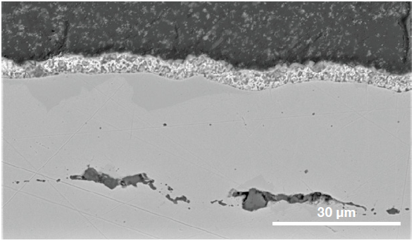
Figure 8. Cross section of the steel showing the coatings involved and the presence of sub-surface inclusions. (Acc voltage 15 keV, beam current 0.44 nA). Image Credit: Thermo Fisher Scientific – Electron Microscopy Solutions
Additional characterization of the RoI’s cross section was performed, for this reason, confirming the presence of sub-surface inclusions (Figure 8).
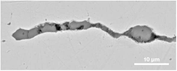
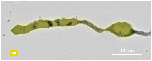
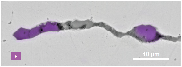
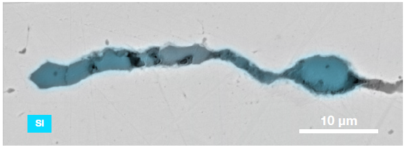
Figure 9. ChemiSEM images of one of the sub-surface inclusions. From top left: backscattered electron image, calcium, fluorine, and silicon maps showing their distribution within the inclusions (Acc voltage 15 keV, beam current 0.44 nA). Image Credit: Thermo Fisher Scientific – Electron Microscopy Solutions
The use of Axia ChemiSEM to characterize one of the sub-surface inclusions revealed the presence of the foreign particle on the surface, as well as the presence of notable amounts of calcium, silicon and fluorine (Figure 9).
Conclusion
Vehicle manufacturers are highly focused on ensuring consistently high durability and corrosion resistance of automotive exposed steel panels, for example, doors, roofs and quarter panels.
Each of these components is required to offer guaranteed high resistance to atmospheric corrosion while maintaining optimum performance for many years.
Final products are always inspected to ensure that they do not present defects in any of the protective coating layers. If these do present defects, further characterization must be performed to understand the underlying cause of the defect and prevent this from occurring in the future.
This article presented a procedure enabling the rapid detection and investigation of foreign particles, as well as the rapid, straightforward assessment of their composition.
Unlike conventional SEMs, the Axia ChemiSEM provides immediate access to all necessary elemental information for accurate defect discovery and failure analysis.

This information has been sourced, reviewed and adapted from materials provided by Thermo Fisher Scientific – Electron Microscopy Solutions.
For more information on this source, please visit Thermo Fisher Scientific – Electron Microscopy Solutions.