An Introduction to Particle Characterization
Particle characterization plays a critical role across a wide range of industries, including pharmaceuticals, chemicals, additive manufacturing, energy, and materials science. Understanding particle properties such as size and shape is essential because these characteristics directly influence material behavior, product performance, and process efficiency.
While particle characterization can include surface texture, porosity, and composition, particle size and particle shape are typically the most influential and most commonly measured parameters. A deeper overview of how these properties are defined and used in industry can be found in this guide to particle characterization fundamentals.
Why Particle Size and Shape Matter
Particle size affects many material properties, including dissolution rate, flowability, packing density, filtration efficiency, and reactivity. However, particle shape often plays an equally important role. Two particles with the same equivalent diameter may behave very differently if one is spherical and the other is elongated or irregular.
This is why modern particle characterization increasingly focuses on measuring both size and shape together, rather than relying on a single diameter value. A more detailed discussion on how particle shape influences size measurements and material behavior is available here:
How particle shape impacts size results.
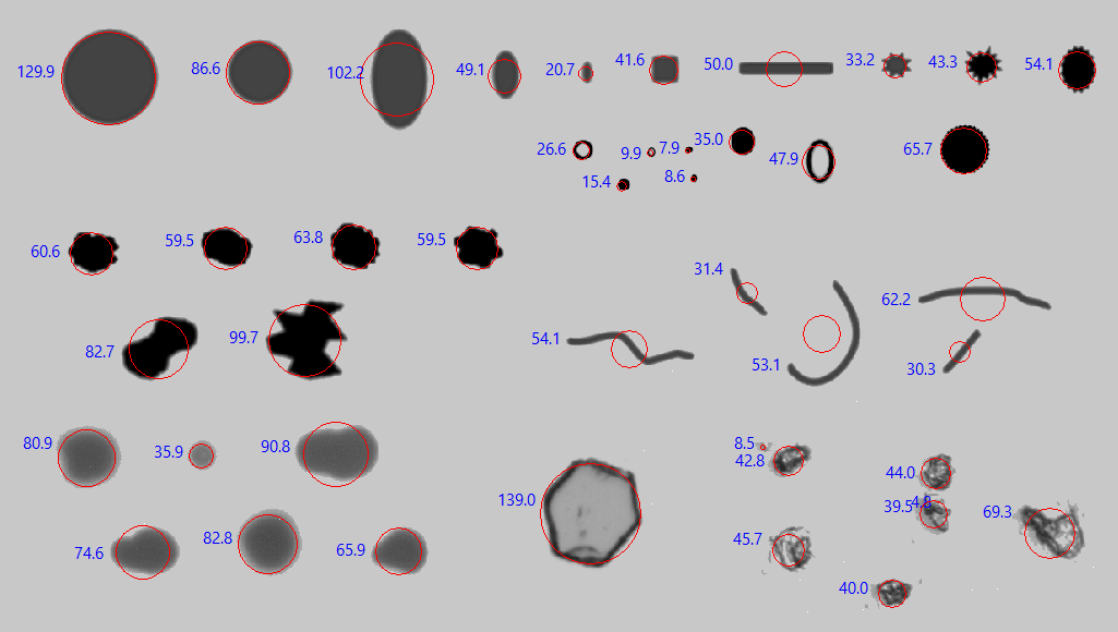
Figure 1. Example images of particles with similar equivalent diameters but different shapes, illustrating how shape can influence material behavior and measurement results. Image Credit: Vision Analytical Inc.
Distribution Histograms
To illustrate statistical results from sample analysis, particle data are divided into classes or “bins,” and the number of particles in each size bin is reported. Particle size information can be displayed in number-weighted, volume-weighted, or surface-area-weighted histograms, each providing different insights into the sample composition.
Because dynamic image analysis identifies and measures individual particles, statistical histograms are particularly accurate. These histograms allow users to see exactly how many particles fall into each bin, and - in imaging systems - to view thumbnail images of particles that back up the statistical results.
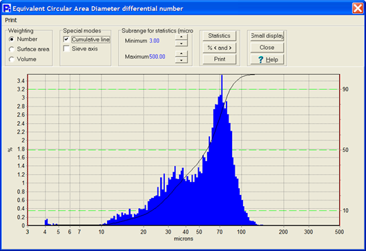
Figure 1 - A number-weighted size histogram showing the presence and quantity of fine particles in a sample. Image Credit: Vision Analytical Inc.
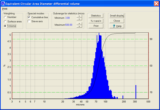
Figure 2 - A volume-weighted size histogram is equally important to view of your sample to get a view of the presence of large particles such as contamination and agglomerates. Image Credit: Vision Analytical Inc.
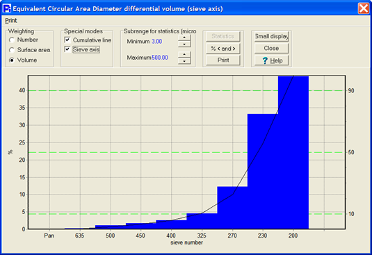
Figure 3 - A sieve correlation size histogram, typically used to compare traditional sieve data with automated measurement methods. Image Credit: Vision Analytical Inc.
Interpreting Distributions
Users should view, at a minimum, both number-weighted and volume-weighted distributions. Number-weighted distributions highlight fine particles, which may clog filters or affect flow properties, while volume-weighted distributions that are statistically graphed based on each particles volume calculation will emphasize larger particles that can show important factors such as agglomerates, or even bubbles.
Surface-area-weighted distributions are also useful when surface phenomena are important, such as in catalysis or coatings. However, surface-area calculations do not account for porosity; specific porosity measurements require dedicated instrumentation.
The following chart explains why one sample can have different number-weighted and volume-weighted histograms. This also shows the benefit of always studying both weighted statistics and using both to compare and contrast. The number and volume weighting can offer value in observing small quantities of agglomerates (larger particles) by reporting by volume and a higher number of fines (smaller particles) reporting by number.
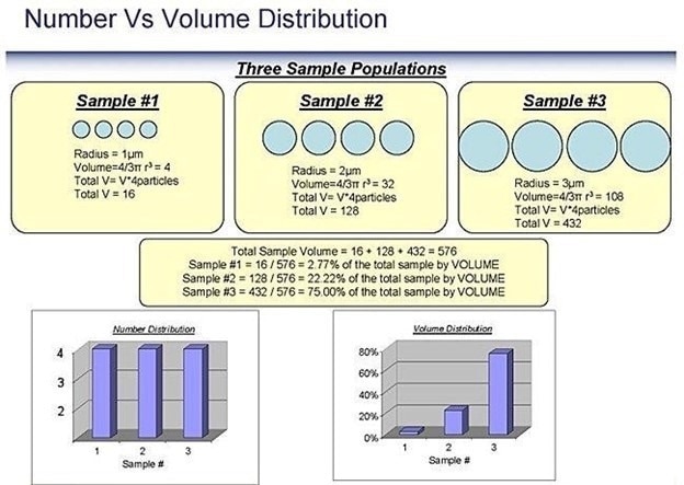
Figure 4 - Comparing a number weighted distribution to a volume weighted distribution. Both are important to view from automated particle analysis results. Image Credit: Vision Analytical Inc.
Shape and Fraction Measures
In some cases, particle shape measurements are size-independent. Fractions such as circularity or aspect ratio give numerical values between 0 and 1 - where values closer to 1 indicate shapes that are more regular or circular.
When both size and shape information are needed to characterize a complex sample, advanced techniques such as dynamic image analysis are often used. For a deeper explanation of how size and shape data are combined and interpreted, see how particle shape impacts size results.
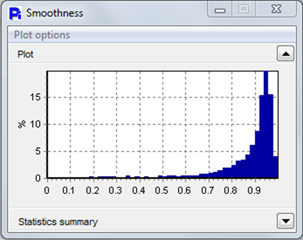
Figure 5 - Example histogram showing the shape fraction distribution for perimeter smoothness. This is a critical factor to know if the flowability or packing density of your sample is important. Surface irregularity impacts this greatly. Image Credit: Vision Analytical Inc.
More on Statistics
A typical statistical result not only gives the graphical histogram, but also will report a large amount of data. Below is a sample of a size-based histogram and associated data.
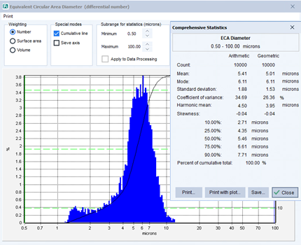
Image Credit: Vision Analytical Inc.
Typical size distribution is characterized by different values. One of the most common being the mean size. A mean value allows some information of the particle size but does not issue any indication about the shape of the distribution or how broad or narrow it is. The number or arithmetic mean is purely the average value. It is frequently denoted as D1,0. Other means take into account volume weighting and area.
Assuming sphericity of particles, the generic definition of a weighted Dp,q mean diameter is:
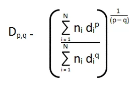
Image Credit: Vision Analytical Inc.
Definition of Dp,q means
The diameter means that are most often of use in characterizing a particle sample are:
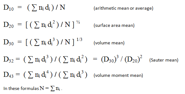
Image Credit: Vision Analytical Inc.
In these definitions, ni is the count in size bin number i, and di is the representative diameter of that size bin. The sums are over all particles, and N is the particle count total.
Descriptions of these means in words are as follows:
Arithmetic mean diameter, D[1,0] : the average of the diameters of all the particles in the sample.
Surface mean diameter, D[2,0] : the diameter of a particle whose surface area, if multiplied by the total number of droplets, will equal the total surface area of the sample.
Volume mean diameter, D[3,0] : the diameter of a particle whose volume, if multiplied by the total number of particles, will equate all the sample’s volume.
Surface moment mean diameter, D[3,2] (“Sauter mean”): the diameter of a particle whose ratio of volume to surface area is the same as that of the complete sample. Mathematically, if V is the total volume and A is the total surface area of the sample, D3,2 = 6 * (V / A).
Volume moment mean diameter, D[4,3]. This value is an indicator weighted on the volume of particles. This is the mean value that is most used by Laser Diffraction instrumentation.
The Mode is the most frequent size present.
The Harmonic mean is N / Σ (ni / di)
Geometric Means
Geometric means reflect the visual weighting of a log-size axis. The geometric mean diameter will appear as the center of a distribution on a log scale, while the usual arithmetic mean may sit a lot lower on the size scale (as smaller sizes are a lot more numerous than larger sizes).
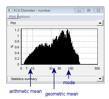
Image Credit: Vision Analytical Inc.
To compute the geometric mean, use the logs of the x-axis values ( log (di) in place of di ) :
The Geometric mean is Σ [ni log(di)] / N
With the use of the same manner, the geometric versions of the other means and standard deviation may be calculated.
Measures of Spread
Standard deviation measures how wide the distribution is:
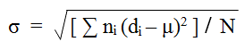
Image Credit: Vision Analytical Inc.
where μ = mean diameter (D10). It has units of microns (for a size distribution).
The Coefficient of Variance is the ratio of the standard deviation to the mean: CV = σ / μ . To express as a percent multiply by 100. Being a ratio, this statistic does not have units.
Percentiles
Percentiles are a way of conducting size information as one or more numbers. The Median size splits the particles into two parts containing equal counts. Strictly speaking, this is the Number Median. It is also known as the 50th or the 50% percentile.
The 10th percentile defines the size with the property that 10% of the particle count is less than that size. Any other percentile can be defined similarly. Commonly, three percentiles (10%, 50% and 90%) are used as a characterization that is uncomplicated but provides additional information to a single mean. Additional percentiles are available and customizable in the Insight software to meet the needs of any specific industry requirement.
The Volume Median, or 50th percentile by volume, splits the volume of the sample into two equal pieces. The two classes will hold equal volume but not an equal count of particles. Other volume percentiles are defined similarly; as an example, the 25th volume percentile is the size such that particles smaller than that size are representative of a quarter of the volume.
Other Characterizations
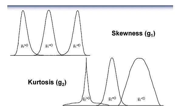
Image Credit: Vision Analytical Inc.
Skewness is an indicator of how asymmetrical the shape of the distribution is, about the center. A positive value will mean there are further counts on the right side of center, normally in the appearance of a tail. A negative value will mean it tails to the left.
Skewness = Σ ni (di – μ)3 / (σ3 N) (σ = std. dev., μ = mean)
Kurtosis is an indicator of how much the shape differs from the typical bell curve in a vertical sense.
Kurtosis = [Σ ni (di – μ)4 / (σ4 N)] / - 3 (σ = std. dev., μ = mean)

This information has been sourced, reviewed and adapted from materials provided by Vision Analytical Inc.
For more information on this source, please visit Vision Analytical Inc.