Particle analysis is a crucial step in the quality control of bulk materials and is performed in laboratories worldwide. The methods used have usually been established for years and are rarely questioned.
Regardless of these facts, the procedure should be periodically critically reviewed because a wide range of sources of error can negatively impact the results of particle analysis.
This article discusses the pros and cons of various methods of particle characterization and explains how to make them more reliable and accurate.
1. Sampling
When sampling inhomogeneous bulk materials, it is important to ensure that the properties of the sample taken in the laboratory correspond to those of the total quantity. This is called representative sampling. The fact that during handling materials separate by size (segregation) can make correct sampling difficult.
For example, vibration causes small particles to move down the interstitial spaces and gather at the bottom of the container during transportation. In bulk cones, concentration of the small particles inside the cone is typical.
Therefore, it is hardly representative to only take a sample from a single location. Subsamples are usually obtained from a number of locations and combined to counteract the effect of segregation. The situation can also be further improved by using suitable aids such as sampling lances.
2. Sample Division
For particle analysis, the sample amount available is generally too large for the measuring instruments used. Consequently, the quantity must be reduced further in the laboratory. Poor or unperformed sample division is one of the primary sources of error in particle analysis, particularly for materials with wide size distributions.
Random sampling creates subsamples with varying particle distributions, which can be observed in the poor reproducibility of the measurement results (Fig. 1a).
The use of sample dividers can correct this situation. Reproducibility can be significantly improved using a simple sample splitter when several subsamples are analyzed.
Automatic rotating sample dividers, such as the Retsch PT 100, deliver the best dividing results (Fig. 1b). The sample material used is a standard sand with a particle size between 63 µm and 4000 µm. The blue and black * represent the reference values.
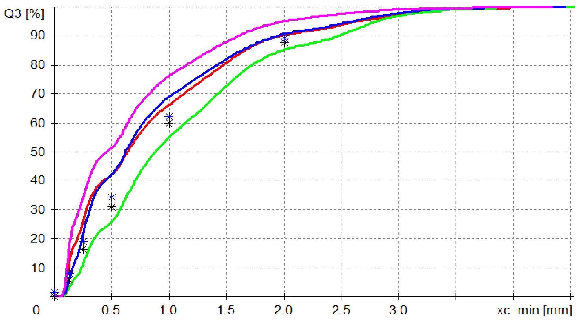
Figure 1a. Random sampling. Four measurements with the CAMSIZER P4 image analyzer (red / blue / violet / green) provide four different results. None is within the expected range (black and blue *). Image Credit: Microtrac MRB?
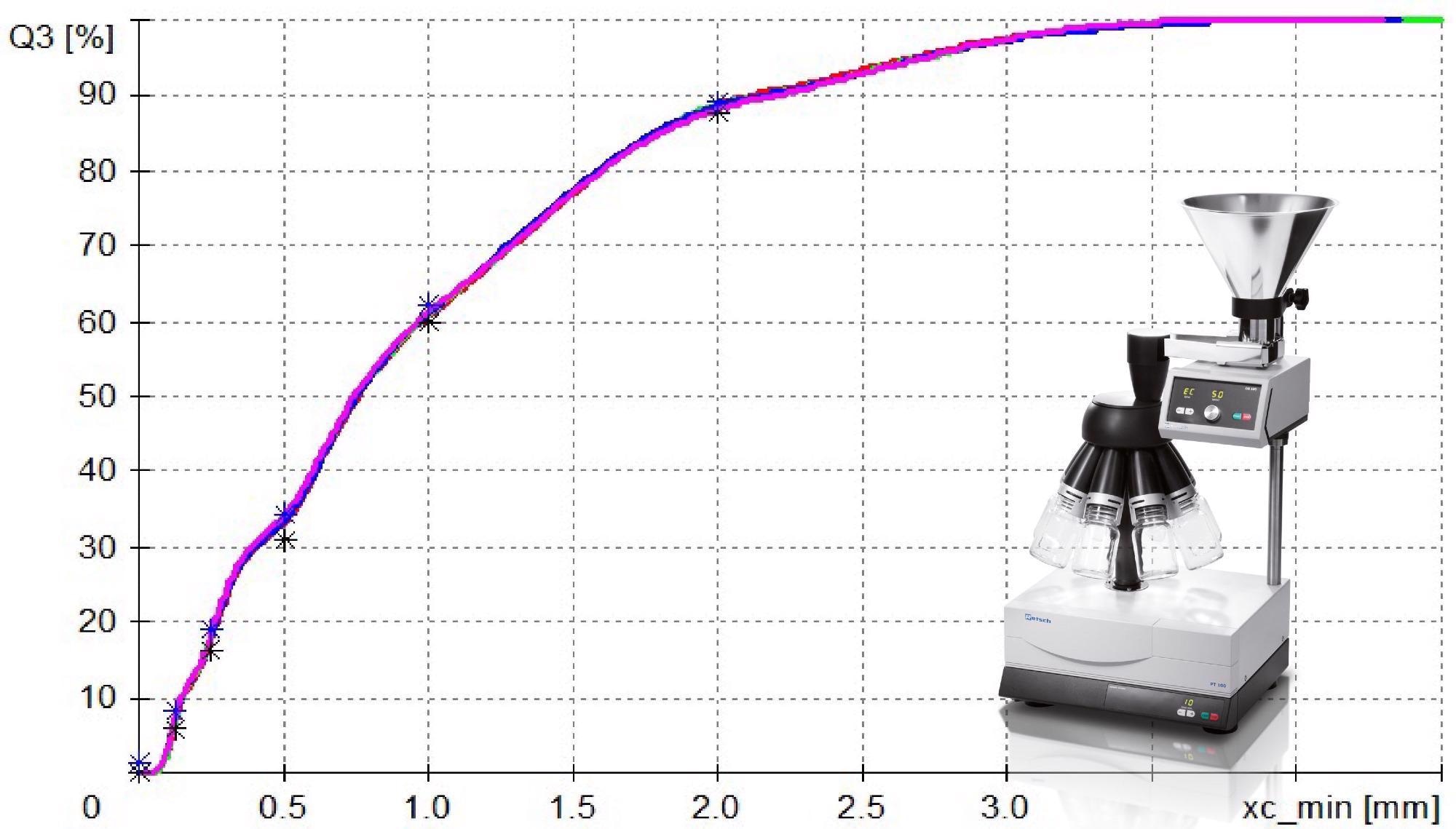
Figure 1b. Sample division with rotating sample divider provides four identical and correct results. Image Credit: Microtrac MRB?
3. Dispersion
Dispersion is the separation of particles to make them easy to measure. Particles that cling to one another as a result of various attracting forces are called agglomerates. It is recommended to break up these agglomerates prior to taking measurements.
However, it may also be worthwhile to create agglomerates in a targeted manner (granulation). In such cases, proceed with dispersion carefully to not destroy the structures prepared for measurement.
For dry measurements, dispersion is generally conducted in a compressed air stream. Figure 3 shows an example of dry measurements using the CAMSIZER X2 at different dispersion pressures.
In the first example (Fig. 3a), as the pressure rises, the result becomes increasingly finer until it stabilizes around 150 kPa and above. Therefore, for this sample, 150 kPa would be the optimum dispersion pressure.
Generally, when selecting the dispersion pressure the rule applies ”as much as necessary and as little as possible”. For the majority of powdered materials, 20-30 kPa is sufficient for complete dispersion.
In the next measurement example (Fig. 3b), the dispersion becomes increasingly fine from a pressure of 100 kPa, which indicates that the particles are ground. Pourable samples may even be analyzed in free fall.
Agglomerates can also appear in suspensions. This can usually be avoided by choosing an appropriate dispersing medium (carrier fluid). Agglomerates that are still present in the suspension can be separated using ultrasound.
Most advanced particle sizers have integrated powerful ultrasonic probes, so that sample preparation can be performed entirely inside the instrument (Fig. 4).
Generally speaking, the larger the particles, the greater the probability of error in sampling and sample splitting. With finer particles, the error is more likely to happen during the dispersion phase.
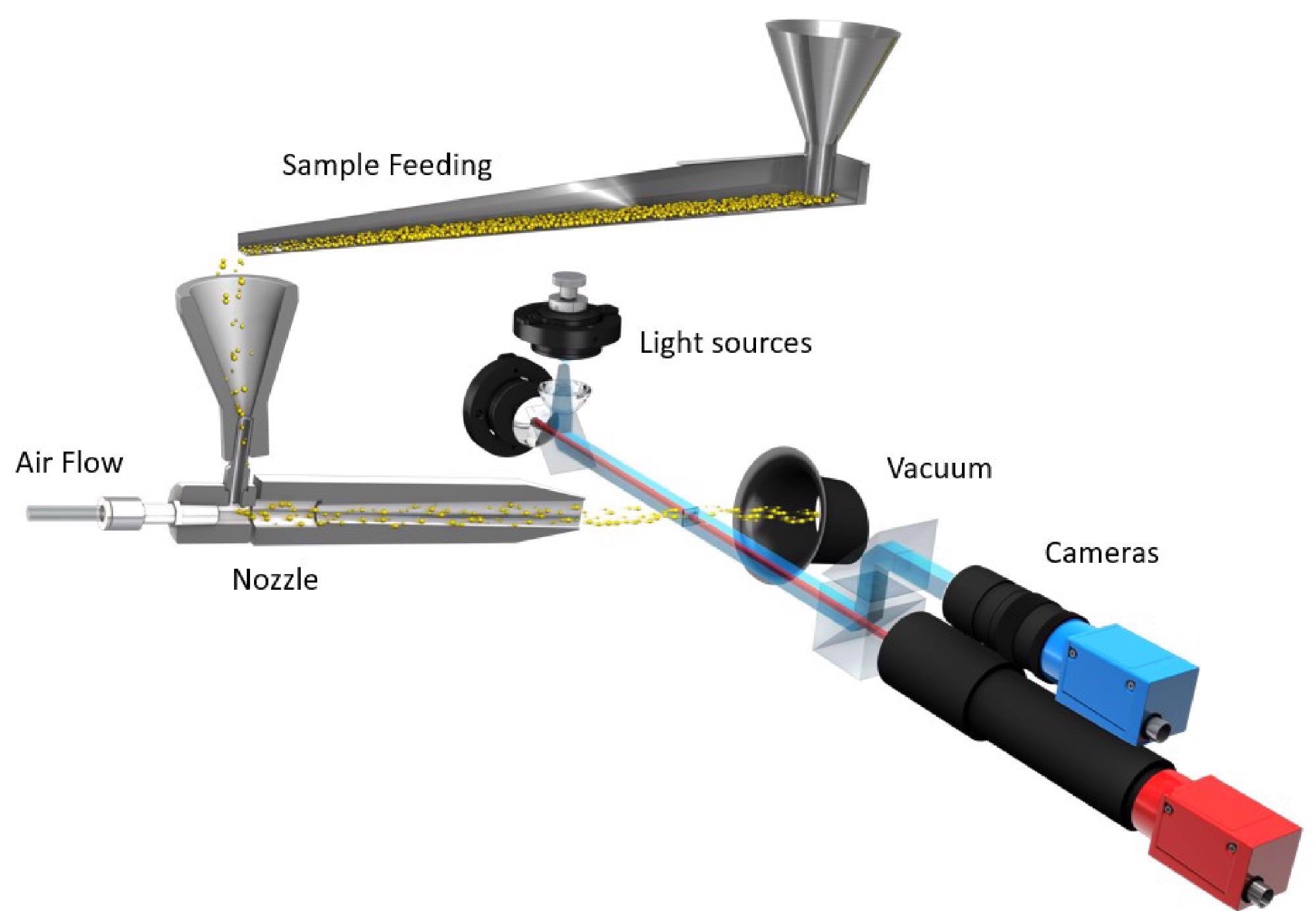
Figure 2. The dry dispersion module of the CAMSIZER X2. Image Credit: Microtrac MRB?
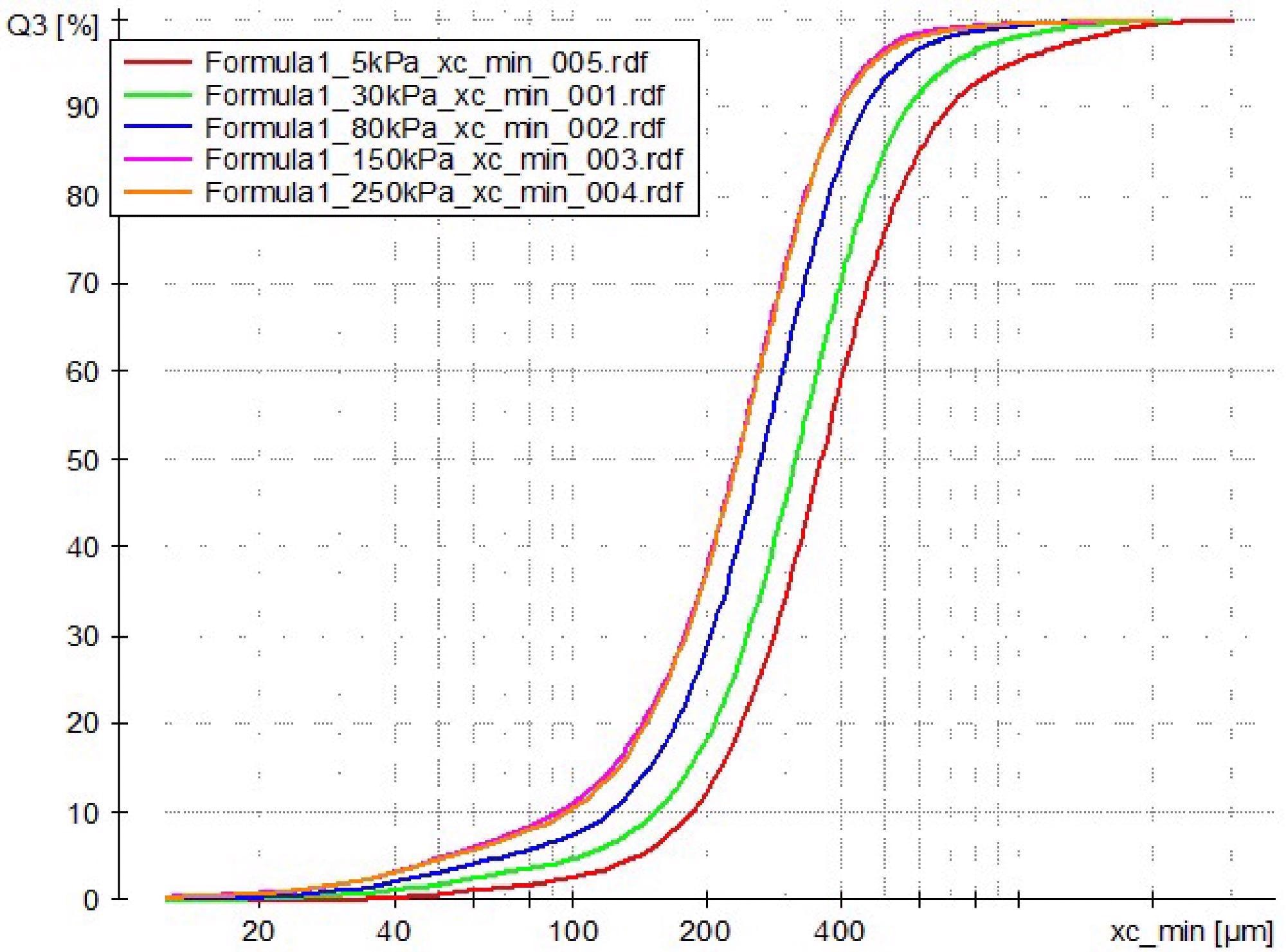
Figure 3a. The result becomes finer with increasing pressure. 5 kPa (red), 30 kPa (green), 80 kPa (blue), 150 kPa (violet) and 250 kPa (orange). No change can be detected from 150 kPa to 250 kPa. Sample: milk powder. Image Credit: Microtrac MRB?
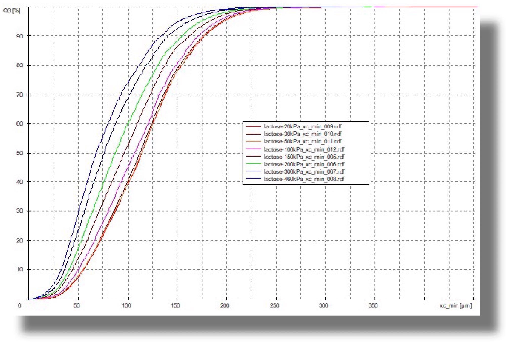
Figure 3b. Measurements at 20 to 50 kPa yield identical results, from 100 kPa the result becomes finer, indicating progressive destruction of the particles. 20 kPa (red), 30 kPa (brown), 50 kPa (orange), 100 kPa (violet), 100 kPa (purple), 150 kPa (gray), 200 kPa (green), 300 kPa (dark green) and 460 kPa (blue). Image Credit: Microtrac MRB?
4. Size Definition
Strictly speaking, particle size is only clearly defined for spherical structures, namely as the diameter of a particular sphere. For non-spherical particles, various measured values can be acquired, depending on the measuring technique used and the orientation.
In the example in Fig. 4, the sphere and Lego brick can pass through a 16 mm sieve, while they are impeded by a 14 mm sieve. For sieve analysis, both objects are equal in size, they have an ‘equivalent diameter’ of 14-16 mm, it is not possible to achieve greater precision with sieve analysis.
When measuring with the caliper, smaller or larger values are acquired, depending on the orientation.
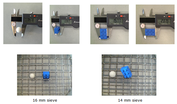
Figure 4. Particle size also depends on the shape and the measuring equipment used. Image Credit: Microtrac MRB?
Even advanced, state-of-the-art particle measurement methods employ different ‘size models’. Ideally, in sieve analysis, particles orient themselves so that their smallest projected area passes through the smallest possible mesh.
Therefore, sieve analysis generally determines the width of a particle. In imaging techniques (e.g., as used by CAMSIZER), various size definitions can be achieved. Size distributions can be separately recorded for length and width.
During laser diffraction, all diffraction signals are assessed as if they were produced by ideally spherical model particles. In contrast to image analysis, in laser diffraction the particle shape cannot be identified.
Furthermore, laser diffraction evaluates a signal generated by a particle collective with particles of different sizes. Calculation of the size distribution is therefore indirect.
Nevertheless, laser diffraction is a well-established technique owing to its exceptional versatility and extensive measurement range from just a few nanometers to the low millimeter range.
Fig. 5 shows the result of the size measurement of coffee powder as a result of sieving, CAMSIZER image analysis, and also laser diffraction.
From the above considerations, it is inevitable to conclude that various methods for particle measurement produce different results.
While it is difficult to correlate laser diffraction and sieve analysis, the results of sieve analysis and image analysis are generally close together, since imaging techniques can identify particle width and sieve analysis is usually a width-based measurement.
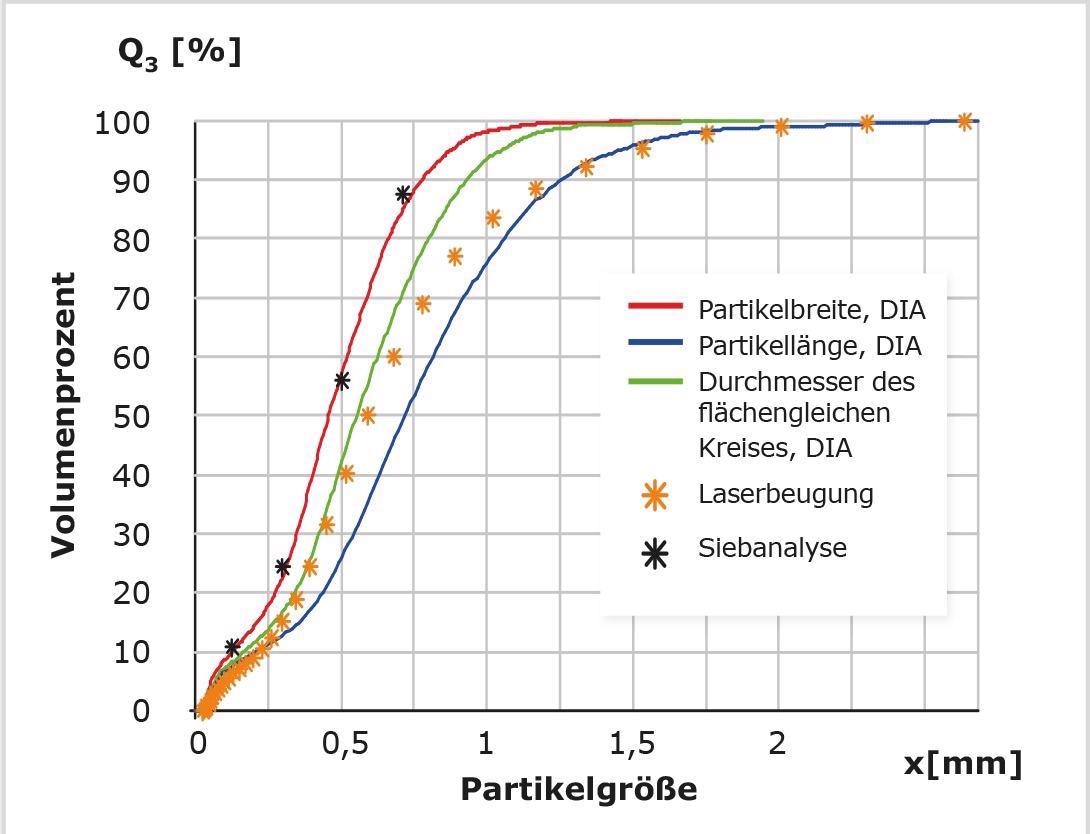
Figure 5. Particle size distributions of a sample of coffee powder determined with sieve analysis (black *), laser diffraction (orange *) and dynamic image analysis. Image analysis provides three results based on particle width (red), particle length (blue) or circle equivalent diameter (green). The definition "width" fits well with sieve analysis, laser diffraction tends to correspond to circle equivalent diameter. Image Credit: Microtrac MRB?
5. Incorrect Sample Amount
Using too much or too little material can negatively impact the measurement result. In laser diffraction, a particle concentration that is too high can create multiple scattering, and if too little sample is used, the signal-to-noise ratio is insufficient.
However, modern laser analyzers signal the optimal concentration measurement and alert users when the amount is too high or too low. In image analysis, you can't actually use too much sample.
Conversely, if too little sample is analyzed, the result will be inconsistent and poorly repeatable due to the small number of detections.
Since the required amount of particle detections is dependent on the size of the particles, and even more so on the distribution width, it is hard to give a general recommendation.
Repeatability tests can be useful, especially when observing the ‘rough end’ of the distribution. Enhanced repeatability can be achieved by using more sample.
In dynamic image analysis using CAMSIZER instruments, a sufficient number of particles are detected in 2-5 minutes under standard conditions to acquire a reliable measurement result.
The greatest influence of sample quantity is in sieve analysis: one of the most frequently seen errors is overloaded sieves. If too much of a sample volume is used, particles can get caught in the meshes and obstruct the sieve. Small particles can no longer pass through the blocked sieve and the measured size distribution is deemed ‘too coarse.’
In sieve analysis, it is necessary to adjust the sample weight in accordance with the particle size and density, as well as the sieve stack used.
Taking the easy way out and always using 100 grams tends to lead to a dead-end, because 100 grams can sometimes be too much or too little. In no case is a representative sample division achieved when weighing 100 g.
6. Underestimating Tolerances
Every measuring instrument demonstrates certain systematic uncertainties and tolerances which must be considered when interpreting the results. Using the example of sieve analysis it is possible to illustrate this point here.
Test sieves are manufactured using wire cloth in line with the standards DIN ISO 3310-1 or ASTM E11. These standards determine how the real mesh size of each sieve is to be tested.
Using an optical method, each test sieve is assessed before delivery and a specified number of meshes are then measured. The average value of the measured opening width must correspond to predefined tolerances around the nominal mesh size.
For a sieve of nominal mesh size 500 µm, the mean value of the real mesh size must be within an interval of +/- 16.2 µm. A sieve conforming to the standard can therefore have an average opening width of between 483.8 µm and 516.2 µm.
It is crucial to note that these are average values; some openings can be even greater and allow particles of a corresponding size to pass through the sieve. Therefore, the standard also determines the maximum aperture size allowed for each sieve size.
Calibration certificates can be obtained for each sieve that supply the relevant information on the actual mesh sizes and their statistical distribution.
7. Overestimating Sensitivity
A common issue in particle analysis is the identification of oversize particles, i.e., a small number of particles that are larger than the main part of the distribution. Here, measurement method sensitivity plays a decisive role.
Imaging methods provide the advantage that each particle detected constitutes a ‘measurement incident’ and is consequently exhibited in the result. For example, this means that the CAMSIZER X2 can determine oversized particle contents of less than 0.02%.
Laser diffraction is a collective measurement method, i.e., evaluation of a scattered light signal simultaneously generated by all particles. The contributions of the individual particle sizes are superimposed, and an iterative procedure is used for the size distribution calculation.
If the number of oversize particles is small, the contribution of these particles is insufficient (signal/noise ratio) to appear in the result. For detection of oversize particles with laser diffraction that can be relied on, the contribution should be >2%.
Microtrac's SYNC laser diffraction analyzer delivers enhanced detection capabilities for oversize particles, as the SYNC has an integrated camera that identifies oversize particles with a high probability of detection.
8. Wrong Density Distribution
Particle size distributions can be graphically represented in a number of ways, with the particle size always appearing on the x-axis.
The histogram representation is intuitively easy to access, where the bar width serves as the lower and upper limit of the measurement class and the height is relative to the number of particles in the respective size interval.
These size intervals are generally established by utilizing the performance and resolution of the measurement system used. While a sieve stack of 8 sieves results in 9 size classes (the sieve bottom counts), image analyzers generate several thousand measurement classes, and laser diffraction analyzers produce 64-150 classes, depending on the configuration of the detector.
Further information content is provided by the cumulative curve here, which exhibits the summation of the quantities in each measurement class. This yields a curve that continuously rises from 0% to 100%.
For each x-value (size), the number of particles smaller than x can be read from the cumulative curve. Additionally, the cumulative curve displays the percentiles directly, such as the d50 value (median).
Popular with a large proportion of users is the representation as distribution density, often incorrectly and succinctly referred to as a ‘Gaussian curve’.
The distribution density is the first derivative of the cumulative curve. The density distribution has a maximum where the cumulative curve rises steeply; the density distribution has a minimum where the cumulative curve is flat.
Therefore, it is crucial that a true density distribution displays the slope of the cumulative curve. Hence, it is necessary to divide the quantity in the measurement class by the class width.
The accuracy of the density distribution increases with the number of measurement classes. The procedure of joining the bars of the histogram by a ‘balancing curve’ does not produce a density distribution.
As a result of the low information content and the error-proneness of the density distribution, it is recommended to dispense with it in favor of a cumulative distribution.
9. Types of Distribution (Number, Volume, Intensity)
Particle analysis results are generally given as a percentage, either as a percentage per measurement class, or as a proportion larger or smaller than a particular size x.
However, these percentages can wildly vary in meaning. It makes a significant difference as to whether these values pertain to mass, volume, or number. Which type of distribution is present depends heavily on the measuring system being used.
In sieve analysis, the weights of the sample in each fraction are established by back-weighing and are then converted into mass percentages. These are equivalent to a volume-based distribution, as long as there are no density differences between particles of different sizes.
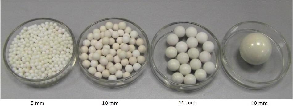
Other methods, such as hand measurement with a caliper, offer number-based distributions predicated on an amount of particles in each measurement class. The difference between mass/volume-based and number-based distributions is displayed in Fig. 6.
For volume distributions, large particles possess a stronger weighting, while for number distributions, small particles are weighted stronger.
Laser diffraction connects all signals to a sphere of equal effect and therefore delivers volume-based distributions. Laser diffraction cannot identify number distributions due to the fact the evaluation is of a collective signal and not individual incidents.
The situation differs for single particle measurement methods, such as image analysis. In this instance, the measurement data are mainly distributed based on a number.
While microscopic methods (static image analysis) generally work with number distributions, it is standard practice in dynamic image analysis to convert to volume distributions.
Since image analysis represents different size definitions, it is possible to conduct this conversion with reliability using a suitable volume model (typically a prolate rotational ellipsoid).
This makes image analysis data comparable to sieve data or laser diffraction. Converting laser diffraction results to number distributions is also possible, but since only a simple spherical model is available, this is less precise, and it is recommended that the volume distribution should be used when possible.
Dynamic light scattering depicts a special case where particle sizes are weighted based on their contribution to the overall scattering intensity. This results in large particles being represented strongly in the result.
This occurs because the scattering intensity expands with size by a factor of 106, which indicates that a 100 nm particle scatters a million times more photons than a 10 nm particle.
In DLS, it is customary to alter distributions to ‘volume-based’, but when interpreting the results, care must be taken to establish which distribution type was used.
| Size (mm) |
Weight (g) |
P3 (%) |
Number |
P0 (%) |
| 5 |
190 |
25 |
490 |
85.5 |
| 10 |
190 |
25 |
64 |
11.2 |
| 15 |
190 |
25 |
18 |
3.1 |
| 40 |
190 |
25 |
1 |
0.2 |
| Total |
760 |
100 |
573 |
100 |
Figure 6. Difference between number- and mass-based distribution using the example of four different grinding ball sizes. In the volume- or mass-related distribution (P3), all fractions are present in equal proportions at 25%. Since the number decreases with increasing particle size, the number-related proportions (P0) are higher in those of the small grinding balls. Image Credit: Microtrac MRB?
10. Working Without SOPs
In particle measurement, as with all other analytical methods, a basic standardized procedure is also necessary for meaningful and consistent measurement results. Such Standard Operating Procedures (SOPs) continually ensure the same, defined measurement processes and work steps.
An essential requirement is that all instrument settings are saved by the software and can be easily retrieved. However, an SOP is made up of more than just instrument settings. Specifications for sampling, sample division, sample preparation and evaluation should also be effectively determined here.
It is recommended that work instructions are published that are as precise and easy-to-follow as possible to ensure measurement results of consistent quality.
Conclusion
When conducting particle analysis several methods may be employed, the most frequently used being laser diffraction, dynamic image analysis, and sieve analysis.
Successful analysis and relevant results can only be acquired if preparatory steps such as sampling, sample division, and sample preparation are performed in the appropriate manner.
The selection of the correct method for the sample material and an appropriate evaluation of the measurement data eventually produces a successful particle analysis.
Microtrac MRB offers the complete portfolio for particle characterization from a single source as one of the major suppliers of particle measurement technology - from the fields of laser diffraction and dynamic light scattering to static and dynamic image analysis.
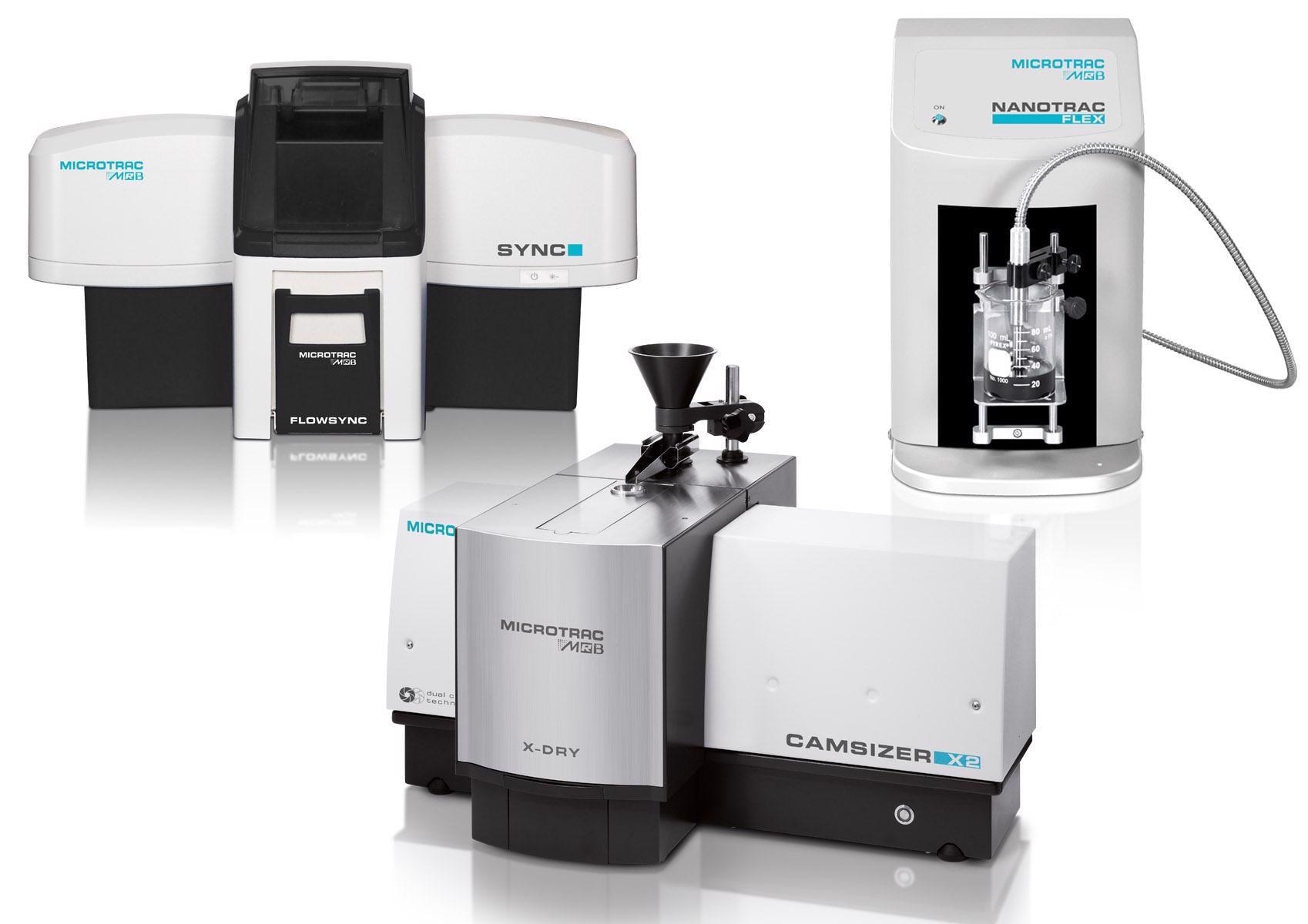
Figure 7. Microtrac MRB's product range for particle size and shape analysis includes techniques such as Dynamic Image Analysis, Laser Diffraction and Dynamic Light Scattering. Image Credit: Microtrac MRB???????
Acknowledgments
Produced from materials originally authored by Dipl.-Phys. Kai Düffels from Microtrac Retsch GmbH.

This information has been sourced, reviewed and adapted from materials provided by Microtrac MRB.
For more information on this source, please visit Microtrac MRB.