How Micro-FTIR Improves Microplastic Particle Identification

When analyzing microplastics (MPs) in real environmental matrices, the plastic particles must be clearly identified with no room for error.^1–7 This is so they can be distinguished from particles of biogenic origin (e.g., particulate organic matter) and particles affiliated with the microlitter in general (i.e., non-plastic artificial and natural fibers, or plastic additives).

Among the standard non-invasive methods to quantify suspected MPs in these matrices, optical microscopy with dye staining and electron and fluorescence microscopy are widely used. However, because they do not provide unambiguous polymer identification, these techniques can be limiting.^8–10

Conversely, vibrational spectroscopy, which leverages Fourier transform infrared (FTIR) and Raman spectrometers, is a recognized non-destructive technique that facilitates the characterization of polymers and other particles.

This means that after the optical investigation has taken place, several particles are selected for further analysis, typically by means of an FTIR spectrometer. The analysis of larger particles or fibers (>500 μm) can be undertaken by attenuated total reflection (ATR)-FTIR since over/underestimation of MPs can occur.

Particle quantification (microscopic counts), followed by the analysis of selected particles for unequivocal identification, is an extremely time-consuming process. Moreover, the analysis of just a few particles may not fully represent what is really going on in the sample.

In contrast, while punctual analysis of particles that employ techniques such as micro-FTIR and micro-Raman can also be time-intensive, micro-FTIR enables the identification of MPs and other microlitter components, especially those below 100 µm (small microplastics, SMPs).

At the same time, it offers reliable microscopic counts for accurate quantification, thus minimizing the chance of over- or underestimation.^3,4,6,11,12 

Particle analysis can be performed using the Particles WIZARD section of Thermo Scientfic^™ OMNIC^™ Picta^™ Software, the built-in software of the Thermo Scientific^™ Nicolet^™ iN10 MX Infrared Imaging Microscope. The analysis can be performed on, and is compatible with, various filter types suitable for the analysis of microplastics, including aluminum oxide filters, silicon oxide filters, etc.

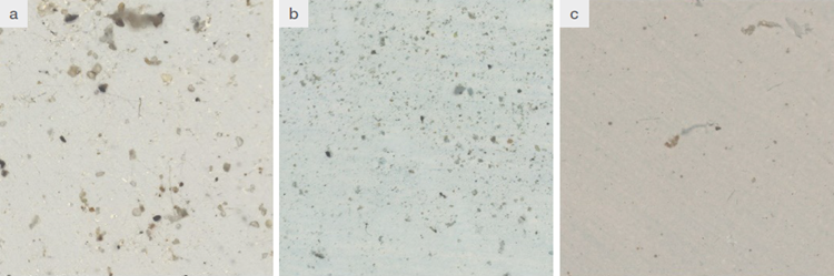
Figure 1. Examples of mosaic or count field: a) in permafrost sample, b) in soil sample, c) in seawater. Image Credit: Thermo Fisher Scientific - Vibrational Spectroscopy

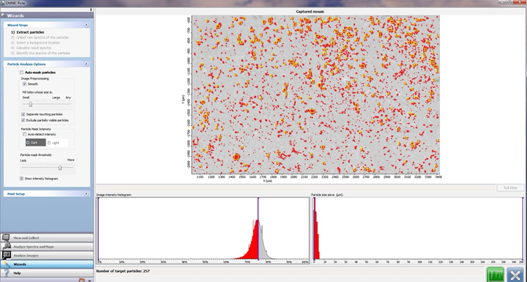
Figure 2. Particle Analysis via WIZARD: Example of how to select the particles on the count field. Image Credit: Thermo Fisher Scientific - Vibrational Spectroscopy

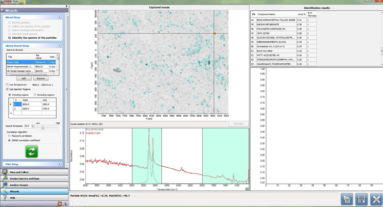
Figure 3. Particle Analysis via WIZARD: The spectra of the particles are identified. Image Credit: Thermo Fisher Scientific - Vibrational Spectroscopy

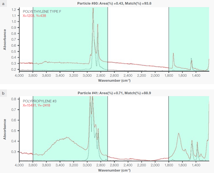
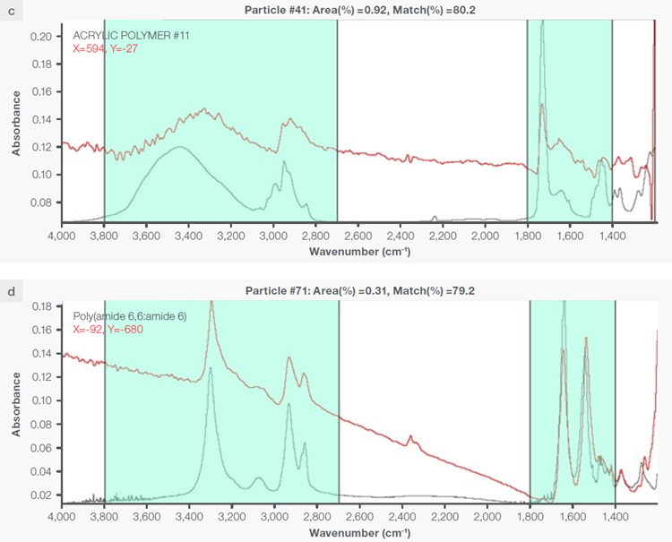
Figure 4. Some exemplary spectra of polymers optimally identified with a match percentage >80%: a) polyethylene, b) polypropylene, c) acrylic, d) polyamide 6. Image Credit: Thermo Fisher Scientific - Vibrational Spectroscopy

Experimental Considerations

Selection of Particles

An area is framed using the objective of the micro-FTIR set to a spatial resolution of 100 µm. Following this, a mosaic of definite dimensions is derived. For instance, in environmental samples, the dimensions applied will typically be 2000 µm x 1400 µm. This mosaic will then act as the “count area” or “count field” (Figure 1).

Once the mosaic is saved, the Particles Analysis function, located in the WIZARD section of OMNIC Picta software, can be initiated. The particles located in the specific count area of the filter’s surface are identified in relation to the brightness value (the brightness ratio of each particle in contrast to the background) defined in Figure 2.

A user’s first port of call is to uncheck the ‘auto-mask particles’ option before selecting ‘smooth,’ ‘separate touching particles,’ and ‘exclude partially visible particles’ in image preprocessing. The latter two are crucial for microscopic counting.

Then, uncheck ‘auto-detect intensity’ in the particle mask intensity menu and select ‘show intensity histogram’. The intensity histogram can then be used to select the particles for later analysis. The particles are contained within rectangles known as bounding boxes.

Since the amount of microplastics in that field is not known beforehand, the image intensity histogram is required to select an appropriate number of particles. The particle-size sieve function allows any potential interference signal to be reduced (Figure 2); when spectral or background interference is present, the brightness ratio will be impacted, leading the software to detect a lower number of particles.

Subsequently, raw particle spectra are acquired, and by collecting these spectra, a background location can be selected on the count field. Using both the raw spectra and the background spectra, it is possible to calculate the resulting particle spectra.

Finally, reference libraries are used to comparatively identify the resulting spectra, as a match percentage determines each spectrum of each particle (Figure 3). Moreover, each particle can be easily identified by retrieving the coordinates in the count field.

The instrumental characteristics state that the optimal range of match percentage is ≥65%; however, depending on the pretreatment used, the match percentage can be >80% or even greater (Figure 4).

During the pretreatment phase, all spectral and background interferences should be eliminated, especially when applying a purification procedure throughout the filtration process.^3,4 This makes particle selection more efficient while boosting the identification match percentage of each particle over the entire optimal range.

When the identification match percentage is <65%, it is not possible to optimally identify the particles and therefore they are not counted. This is why the abundance of MPs present is typically underestimated.

Microscopic Counting for Microplastics and Microlitter

Microscopic counting has been used to quantify bacteria, phytoplankton, pollen, spores, and MPs.^{3,4,6,13–22} A major benefit of microscopic counting is that it eliminates doubt surrounding the number of organisms, cells, or particles present within reliable, computable limits and degrees of chance.

Filters, round or square, can be used as a support for counting. Analyzed filter areas (i.e., counting areas or count fields) should represent the total filter area to mitigate any issues related to representativeness and reproducibility.

Representative measurement areas of equal size can be selected on the surface of the filter using the approaches as displayed in Figure 5. The approach used in the Bürker chamber can be extended to square filters.

For MP analysis, a minimum of 20 filtering areas (i.e., count areas or count fields) must be analyzed to acquire meaningful and reliable quantification. Since filter loading is an unknown quantity, count areas exhibiting different particle abundances should be included to prevent issues with extrapolating findings for microplastics, organisms, cells, or bacteria.

This guideline means that the randomized approach without overlapping (Figure 5d) can be determined as the most appropriate.^3,4,5,7 The microscopic count can be considered representative when a sufficiently large number of relevant particles have been analyzed, with the recommended minimum being 4000 particles.

When these two criteria have been met, the microscopic count can be deemed reliable, and consequently, the quantification is not held back by under- or overestimation.

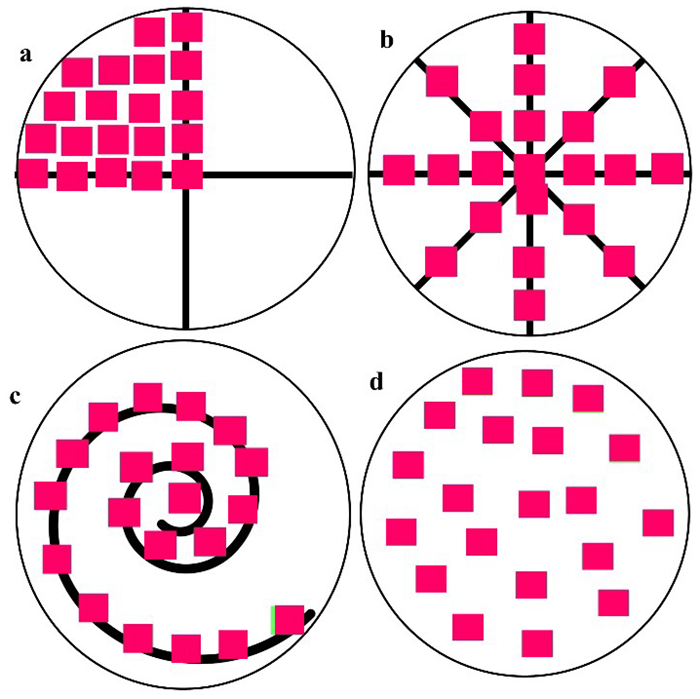
Figure 5. Different approaches may be used for representative measurement areas on filters; at least 20 count areas or count fields should be considered. These approaches can be employed on filters of different diameters and materials (e.g., aluminum oxide, silicon oxide, PTFE). Example a) represents a quarter of the filters; b) represents the cross-section of the four axes; c) represents a helical assembly; and d) represents a randomized assembly. Image Credit: Thermo Fisher Scientific - Vibrational Spectroscopy

The total counts from each filter must be multiplied by the most relevant microscope conversion (optical factor F) and volume or dilution factors to obtain the absolute abundance (number of MPs per liter, kilogram, or meter, etc.).^3,4,5,7 The equations for calculating the abundances are as follows:^3,4,5,7

N_MPs L^-1 = n*1000*F/V

Equation 1

N_MPs kg^-1 = n*1000*F/W

Equation 2

N_MPs L^-1 or N_MPs kg^-1 are the total abundance in the samples analyzed; V is the volume of water analyzed; W is the weight of sediments, soil, etc. analyzed; n is the sum of all the plastic particles in the count fields analyzed; and F is the factor which is calculated as follows:

F = Area of the filter/Area of a count field * number of all the count fields

Equation 3

Selecting and Counting Particles Using WIZARD

Using the WIZARD Particles Analysis function, built into the iN10’s OMNIC Picta software, particles are automatically identified and counted, and the length and width of each particle are also recorded during the analysis.

During particle selection in the software (Figure 1), each particle is outlined with rectangles. These rectangles are known as bounding boxes because they relate to the smallest rectangles surrounding the shape of each particle. The particles’ shapes are then categorized based on the aspect ratio of the bounding boxes.

Calculating the Aspect Ratio and Volume of MPs

The aspect ratio (AR) is calculated as the relationship between the maximum length (L) and the maximum width (W) of the bounding box surrounding the shape: particles are deemed to be spherical when the AR values are ≤1; when AR≥2, particles are categorized as ellipsoidal; and when AR≥3, particles are characterized as cylindrical.

Accordingly, using AR, the volumes of particles and fibers are calculated to be consistent with their geometrical shape (i.e., sphere, ellipse, or cylinder). Once the particles have been reliably identified, it is possible to retrieve information about their density; thus, each particle’s weight can be easily calculated.

AR = L_max/W_max

Equation 4

Conclusions

When analyzing MPs, it is of utmost importance to be able to distinguish the polymers from the rest of the microlitter components and any other particles present in the environmental matrix.

Obtaining an individual analysis of hundreds of particles for reliable quantification can be a time-consuming process, taking up to several days to analyze all FTIR spectra. Moreover, counting MPs separately from vibrational spectroscopy analysis would add a significant amount of time to the analysis, possibly adding as much as running a complete analysis of the entire filter.

Alternatively, in each field count, individual particles are located unambiguously by their unique spatial coordinates. This enables reliable and optimal identification of the spectra, while also collecting the individual particle sizes (width and length).

When switched to Particles Analysis mode, quantification by microscopic count is performed in parallel to spectral identification. Each count field can be saved using the filename extension .map, which facilitates all subsequent analysis of each particle in a precise count field to confirm and validate spectral identification.

Consequently, Particles Analysis software makes the workflow of microplastics analysis considerably less time-intensive and markedly more robust.

Acknowledgments

Produced using materials originally authored by Beatrice Rosso and Fabiana Corami from the Institute of Polar Sciences, and Barbara Bravo from Thermo Fisher Scientific.

References and Further Reading

1. Löder, M.G.J. and Gerdts, G. (2015). Methodology Used for the Detection and Identification of Microplastics - A Critical Appraisal. Marine Anthropogenic Litter, pp.201–227. DOI:10.1007/978-3-319-16510-3_8. https://link.springer.com/chapter/10.1007/978-3-319-16510-3_8.
2. Andrew wirnkor, V., Christian Ebere, E. and Evelyn Ngozi, V. (2019). Microplastics, an Emerging Concern: A Review of Analytical Techniques for Detecting and Quantifying Microplatics. Analytical Methods in Environmental Chemistry Journal, 2(2), pp.13–30. DOI:10.24200/amecj.v2.i2.57. https://www.amecj.com/article_176980.html.
3. Corami, F., et al. (2020). A novel method for purification, quantitative analysis and characterization of microplastic fibers using Micro-FTIR. Chemosphere, 238, p.124564. DOI:10.1016/j.chemosphere.2019.124564. https://www.sciencedirect.com/science/article/abs/pii/S0045653519317886?via%3Dihub.
4. Corami, F., et al. (2021). Small microplastics (< 100 μm), plasticizers and additives in seawater and sediments: Oleo-extraction, purification, quantification, and polymer characterization using Micro-FTIR. Science of The Total Environment, 797, p.148937. DOI:10.1016/j.scitotenv.2021.148937. https://www.sciencedirect.com/science/article/abs/pii/S0048969721040092?via%3Dihub.
5. Corami, F., et al. (2022). Occurrence and Characterization of Small Microplastics (< 100 μm), Additives, and Plasticizers in Larvae of Simuliidae. Toxics, 10(7), p.383. DOI:10.3390/toxics10070383. https://www.mdpi.com/2305-6304/10/7/383.
6. Ivleva, N.P. (2021). Chemical Analysis of Microplastics and Nanoplastics: Challenges, Advanced Methods, and Perspectives. Chemical Reviews, 121(19), pp.11886–11936. DOI:10.1021/acs.chemrev.1c00178. https://pubs.acs.org/chreay/article/121/19/11886/384461/Chemical-Analysis-of-Microplastics-and.
7. Rosso, B., et al. (2022). Quantification and characterization of additives, plasticizers, and small microplastics (5–100 μm) in highway stormwater runoff. Journal of Environmental Management, 324, p.116348. DOI:10.1016/j.jenvman.2022.116348. https://www.sciencedirect.com/science/article/abs/pii/S0301479722019211?via%3Dihub.
8. Möller, J.N., Löder, M.G.J. and Laforsch, C. (2020). Finding Microplastics in Soils: A Review of Analytical Methods. Environmental Science & Technology, 54(4), pp.2078–2090. DOI:10.1021/acs.est.9b04618. https://pubs.acs.org/esthag/article-abstract/54/4/2078/1648219/Finding-Microplastics-in-Soils-A-Review-of?redirectedFrom=fulltext.
9. Ana Violeta Girão (2022). SEM/EDS and optical microscopy analysis of microplastics. In Handbook of Microplastics in the Environment. Springer eBooks, pp.57–78. DOI:10.1007/978-3-030-39041-9_7. https://link.springer.com/rwe/10.1007/978-3-030-39041-9_7.
10. Bai, R., et al. (2023). Microplastics are overestimated due to poor quality control of reagents. Journal of Hazardous Materials, 459, p.132068. DOI:10.1016/j.jhazmat.2023.132068. https://www.sciencedirect.com/science/article/abs/pii/S0304389423013511?via%3Dihub.
11. Mehdinia, A., et al. (2019). Identification of microplastics in the sediments of southern coasts of the Caspian Sea, north of Iran. Environmental Pollution, 258, p.113738. DOI:10.1016/j.envpol.2019.113738. https://www.sciencedirect.com/science/article/abs/pii/S0269749119338382?via%3Dihub.
12. Vianello, A., et al. (2013). Microplastic particles in sediments of Lagoon of Venice, Italy: First observations on occurrence, spatial patterns and identification. Estuarine, Coastal and Shelf Science, 130, pp.54–61. DOI:10.1016/j.ecss.2013.03.022. https://www.sciencedirect.com/science/article/abs/pii/S0272771413001480?via%3Dihub.
13. Andersen, R.A. (ed.) (2005) Algal culturing techniques. Amsterdam: Elsevier Academic Press.
14. Brierley, B., et al. (2007). Guidance on the quantitative analysis of phytoplankton in Freshwater Samples. Available at: https://nora.nerc.ac.uk/id/eprint/5654/1/Phytoplankton_Counting_Guidance_v1_2007_12_05.pdf.
15. Comtois, P., Alcazar, P. and Néron, D. (1999). Pollen counts statistics and its relevance to precision. Aerobiologia, 15(1), pp.19–28. DOI:10.1023/a:1007501017470. https://link.springer.com/article/10.1023/A:1007501017470.
16. Gough, H.L. and Stahl, D.A. (2002). Optimization of direct cell counting in sediment. Journal of Microbiological Methods, 52(1), pp.39–46. DOI:10.1016/S0167-7012(02)00135-5. https://www.sciencedirect.com/science/article/abs/pii/S0167701202001355?via%3Dihub.
17. Huppertsberg, S. and Knepper, T.P. (2018). Instrumental analysis of microplastics - benefits and challenges. Analytical and Bioanalytical Chemistry, 410(25), pp.6343–6352. DOI:10.1007/s00216-018-1210-8. https://link.springer.com/article/10.1007/s00216-018-1210-8.
18. Lisle, J.T., et al. (2004). Comparison of Fluorescence Microscopy and Solid-Phase Cytometry Methods for Counting Bacteria in Water. Applied and Environmental Microbiology, 70(9), pp.5343–5348. DOI:10.1128/aem.70.9.5343-5348.2004. https://journals.asm.org/doi/full/10.1128/aem.70.9.5343-5348.2004.
19. Mazziotti, C., Fiocca, A. and M.R. Vadrucci. (2013). Phytoplankton in transitional waters: Sedimentation and Counting methods. Transitional Waters Bulletin, pp.90–99. DOI:10.1285/i1825229Xv7n2p90. https://ese-journals.unisalento.it/index.php/twb/article/view/13427.
20. Muthukrishnan, T., et al. (2017). Evaluating the Reliability of Counting Bacteria Using Epifluorescence Microscopy. Journal of Marine Science and Engineering, 5(1), p.4. DOI:10.3390/jmse5010004. https://www.mdpi.com/2077-1312/5/1/4.
21. Oßmann, B.E., et al. (2018). Small-sized microplastics and pigmented particles in bottled mineral water. Water Research, 141, pp.307–316. DOI:10.1016/j.watres.2018.05.027. https://www.sciencedirect.com/science/article/abs/pii/S0043135418303956?via%3Dihub.
22. Tong, H., et al. (2020). Occurrence and identification of microplastics in tap water from China. Chemosphere, 252, p.126493. DOI:10.1016/j.chemosphere.2020.126493. https://www.sciencedirect.com/science/article/abs/pii/S004565352030686X?via%3Dihub.
23. Adachi, K. and Buseck, P.R. (2015). Changes in shape and composition of sea-salt particles upon aging in an urban atmosphere. Atmospheric Environment, 100, pp.1–9. DOI:10.1016/j.atmosenv.2014.10.036. https://www.sciencedirect.com/science/article/abs/pii/S1352231014008255?via%3Dihub.
24. Bharti, S.K., et al. (2017). Characterization and morphological analysis of individual aerosol of PM10 in urban area of Lucknow, India. Micron, 103, pp.90–98. DOI:10.1016/j.micron.2017.09.004. https://www.sciencedirect.com/science/article/abs/pii/S0968432817300409?via%3Dihub.
25. Chakrabarty, R.K., et al. (2006). Emissions from the laboratory combustion of wildland fuels: Particle morphology and size. 111(D7). DOI:10.1029/2005jd006659. https://agupubs.onlinelibrary.wiley.com/doi/full/10.1029/2005JD006659.
26. Hamacher-Barth, E., Jansson, K. and Leck, C. (2013). A method for sizing submicrometer particles in air collected on Formvar films and imaged by scanning electron microscope. Atmospheric Measurement Techniques, 6(12), pp.3459–3475. DOI:10.5194/amt-6-3459-2013. https://amt.copernicus.org/articles/6/3459/2013/.

This information has been sourced, reviewed, and adapted from materials provided by Thermo Fisher Scientific - Vibrational Spectroscopy.

For more information on this source, please visit Thermo Fisher Scientific - Vibrational Spectroscopy.