Petroleum product pipelines offer an efficient way of delivering product to distribution terminals. These multi-purpose pipelines deliver several different fuels usually injected into the pipeline in a sequential manner without any physical barriers between products. The receiving terminal should detect and separate the products to send them to the right tanks and should also identify the off-specification product that has to be directed to slop for return to the refinery for reprocessing.
Diesel might be a typical sequence, followed by high octane gasoline, low octane gasoline, fuel oil, and so on. If a product is directed to the wrong tank, it can result in major consequences. Switching excess product to slop decreases profits since a valuable product is lost and added to this, there is the extra cost of reprocessing the slop in refineries.
The Solution
The solution is to distinctly identify the product in real-time as it reaches the terminal thereby facilitating the timing of the switching between tanks. With regards to time, the stream will change from 100% product A through an intermix region to 100% product B. Univariate sensors, for example, gravitometers (densiometers) and refractive index meters are not advanced enough to offer real compositional information about the product and therefore have restrictions on their ability to detect the transition for all product combinations. Process Insights’ Near Infrared (NIR) analyzers can offer direct compositional information that can be used to unambiguously detect the product change as well as identify the product as diesel, gasoline, and so on.
The Smart Choice
Two smart choices are available from Process Insights to solve this issue. The full range NIR-O™ spectrometer can be used to offer almost complete chemical information on the sample. On the other hand, the ClearView™ db multi-wavelength photometer produces more limited information, but would still offer rapid interface detection as well as some chemical information. These instruments employ fiber optic cables and direct insertion probes into the pipe to determine the product as it flows by.
Objective
1) Quantitatively detect the transition from Product A to Product B in the pipeline and hence facilitate the switching from Tank A to slop (mixed product) to Tank B while reducing the slop volume.
2) Explicitly identify the product in the pipeline.
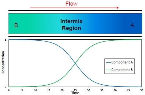
Figure 1. Pipeline Product Flow
As shown in Figure 1, the Product A is injected into the pipeline followed by Product B sometime later. This produces an intermix region between the two products. The goal at the receiving end is to economically change from Tank A to slop and then to Tank B without affecting either Product A or B and to reduce the volume of slop which has to be re-processed.
From a theoretical standpoint, the intermix region is representative of an exponential decay of Product A and an exponential increase in Product B.
Listed below are some common methods presently used for detecting the pipeline product change. At present, these univariate sensors are the best practices in the industry, and they offer very little information regarding the actual product identification
Common Methods Currently Used
- Gravimetric (density) sensors – while these can sense the variation in the product, they cannot identify the product. These may have complexity in detecting the variations between similar products, for example, different grades of gasoline.
- Refractive Index (RI) sensors – a sensitive technique that can easily detect some variations in products, but does not detect all changes. These may be able to detect certain products but measurement is univariate and cannot guarantee that the ID is correct.
- Color analysis – this works only for dyed fuels.
NIR spectroscopy (either full spectrum or discrete wavelength photometers) can offer important information about the product itself and categorize it to different grades of diesel, fuel oil, gasoline, etc. The data described here were obtained using a Process Insights full spectrum NIR analyzer.
Experiment
A pipeline was simulated using current laboratory equipment with sample flowing through 40 feet of tubing to a Process Insights 10 mm multipurpose flow cell. The flow cell was linked to a Process Insights full spectrum NIR analyzer through fiber optic cables. Spectral scans in the region of 1000 nm to 1600 nm were recorded at intervals of 6 seconds. The products employed were 87 pump octane gasoline that included commercial diesel fuel and alcohol.
During the analysis, it was found that gasoline does not always mix well with diesel. One could see layers and sometimes 2-phase flow (globules of one product in the other) in the tubing. A static mixer would have solved these issues, but this was not available.
Algorithm
The strategy is to use NIR spectroscopy to detect the real-time changes in the pipeline material, measure the change, and identify the products. The proposed method will utilize the Match Index (MI) equation. The Match Index is a common spectral similarity measure calculated as the cosine of the angle between two vectors. Here, the pipeline spectra to be compared are the vectors.

Pipeline Simulation
Gasoline and diesel fuel are the products used for the pipeline simulation. Figure 2 shows the NIR spectra of these individual products. The important functional groups are identified. A short aromatic peak is seen in low octane gasoline. The strong CH3 peak in the gasoline denotes that this product is primarily branched paraffins. The gasoline sample also has a band because of the OH group in ethanol (an additive). The diesel sample exhibits no aromatics and about equal amounts of CH2 and CH3, denoting a higher presence of normal paraffins which is common for diesel.
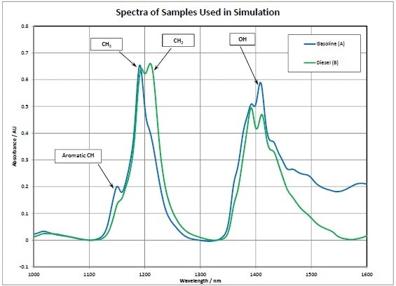
Figure 2. Pipeline simulation, spectral data
Two Simulated Approaches are Studied
- In Case 1: No prior knowledge of what is descending the pipe – A single isolated analyzer should be able to detect the intermix region and measure the changes. A library of potential products is available to the analyzer.
- In Case 2: An upstream analyzer is available possibly at the injection point that can collect a spectrum of product B and transmit that spectrum to the receiving terminal and its analyzer. Therefore, the receiving analyzer knows what is currently in the pipeline and what to anticipate. This makes quantification more accurate and easier.
- Both techniques could gain from having a spectral library of potential products that could descend the pipe. Using this library, the products can be identified and potentially a true least squares or PLS mixture analysis can be carried out. Hence, the operator would know the percentage of product A and B at all times. While that analysis is beyond the scope of this article, it is something that could easily be done.
Case 1 (Figure 3)
Case 1 begins by first choosing a sample (spectrum) that can be used as the reference spectrum in the Match Index calculation. If for instance, the intermix region takes 1 hour to pass through, then the reference spectrum must be collected before 2-3 hours. A new reference spectrum could be chosen every hour to keep it current with the flowing product. Next, the noise in the MI results is calculated. Again this is performed for a period of time 2-3 hours ahead of the initiation of the intermixed sample.
Multiplying the noise by 3 provides 95% assurance that any product below a Match Index of (1- 3σ) is considerably different, thereby providing the first trigger point for switching tanks.
Apart from monitoring the MI value, the derivative of the MI function was also needed to be monitored. The derivative can be approximated by calculating the 1st difference between the samples. Again, the noise during steady-state conditions can be calculated and a 3σ threshold can be determined for the second switching point.
When nearing the intermix region, it could be seen that the MI function decreases drastically, that is, it falls below the 95% confidence limit thereby triggering the switching from Tank A to slop.
It is observed that the derivative (slope) of the MI function has experienced a maximum demoting the rate of change and passed the inflection point in the exponential decay curve for Product A. Additionally, the derivative function was normalized to unity at the inflection point. Thus, it offers a crude direct reading of the degree of mixing of the sample, the peak being approximately 50%.
When proceeding through the intermix region, the MI function levels out and asymptotically reaches a fixed value. When the derivative function falls below its 3σ line, the second switch can be triggered from slop to Tank B with confidence that the sample is statistically not changing anymore.
This experimental setup caused higher noise in the data than what would be expected in a field experiment. This noise is in orders of magnitude greater than the instrumental noise.
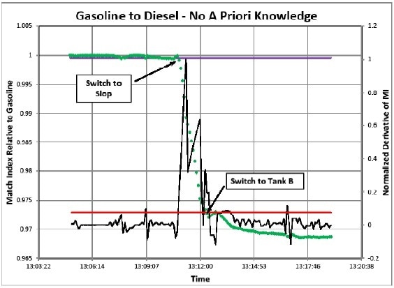
Figure 3. Case 1 Simulation
Case 2 (Figure 4)
Previous knowledge of products in the line – This needs two analyzers—one at the injection point and the other at the terminus with a network link. Analyzer #1 transmits the product spectra in advance so that analyzer #2 can anticipate its reception and more accurately measure the products. A library of potential products is available to the analyzer. In Case 2, there is a prior knowledge of the expected product. Using this prior knowledge, 2 MI values can be calculated with each value for Product A and Product B. Thus, the double exponential curves showed earlier can be traced out. Again, 3σ can be set for both calculations and the switch points can be determined.
An example of the double “S” curve is shown in Figure 4. As the spectrum of both products is known, one could perform a simple least squares fit and actually plot percentages of both products in real time.
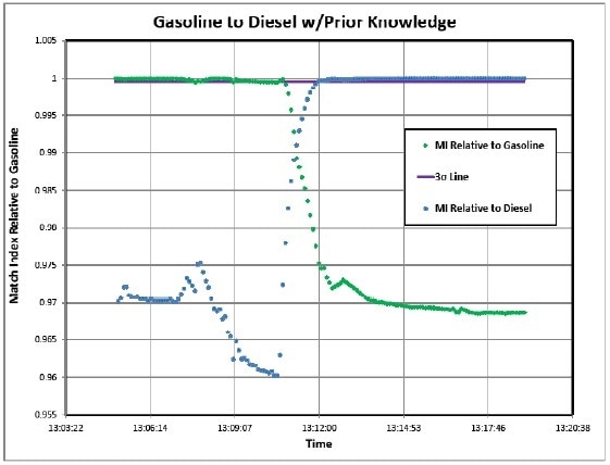
Figure 4. Case 2 Simulation
All of the prior results obtained were for a full spectrum analyzer with >500 individual data points on the wavelength axis. Is it possible to reduce this to just a few wavelengths so that the measurement can be made by a photometer using the previous data? In the earlier data, a simple 2 point baseline correction was made at 1100 nm and 1330 nm. Using peak wavelengths of 1151, 1191, and 1208 nm (shown in Figure 5), the MI calculation was done again.
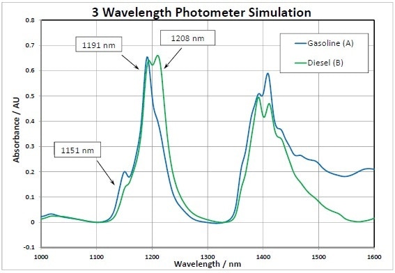
Figure 5. Photometer Simulation
Analysis
A comparison of the MI calculations for full spectrum versus a simulated 3 analytical wavelength photometer is illustrated in Figure 6. Note the similarity of the results. They attain the asymptote at different values for Product B but this is irrelevant because of the nature of the match index calculation and use of the 3σ limit.
Thus, it can be concluded that a simpler alternative, a five wavelength photometer (three analytical wavelengths and two baselines) could actually offer equivalent results at a much lower installation cost. It can be made even more robust by adding a sixth wavelength.
When it comes to identifying the sample from a library, a limited wavelength photometer would not be as accurate as a full spectrum analyzer. However, it still could do a mixture analysis and could operate in Case 1 or Case 2 mode.
Highlights
- Both wavelength photometers and full spectrum analyzers can be used based on the number of measurement points and accuracy levels required
- NIR spectroscopy can quantitatively detect pipeline interface transitions
- The information that can be obtained is considerably greater than what can be obtained with univariate approaches such as RI and gravimetric sensors
- Match Index calculations can compare the present unknown sample with samples in a spectral data base to rapidly identify the sample
- In a similar way, PLS classification is capable of identifying the sample through a scores space calculation, possibly reducing mistakes that send the product to the wrong tank
- Results are available in real-time (seconds)
- Guarantees product quality
- Reduces slop and thus reduces re-processing volume and associated costs
- Increases the quantity of valuable saleable product
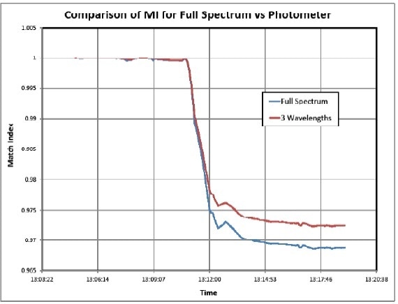
Figure 6. Photometer Simulation Results
Discussion and Conclusions
The pipeline product interface detection methods explained here using Near Infrared (NIR) spectroscopy are both reliable and fast utilizing either the NIR filter photometer or the Process Insights NIR spectrometer. This technique reduces the need for laboratory sample collection. Results are available in real-time (seconds) for transition detection as well as product identification. For more detailed information regarding system specifications, customers can contact a Process Insights technical sales specialist.
Control That Can Be Measured
By teaming up with Process Insights, customers gain the benefit of more than three decades of experience in online process monitoring and stream sample analysis. The entire product range of Process Insights is designed and developed to meet the challenges of the most demanding production environments for control that can be measured by customers.

This information has been sourced, reviewed and adapted from materials provided by Process Insights – Optical Absorption Spectroscopy.
For more information on this source, please visit Process Insights – Optical Absorption Spectroscopy.