Self-regulating systems with feedback loops, i.e., the routing back of the output of a system to its input, have existed since antiquity and have since become an integral part of modern technology.
Over 150 years ago, one of the first attempts to thoroughly describe control loops using feedback took place in James Clark Maxwell’s article, On Governors.1
In control strategies, an open-loop control system refers to a controller whose action is determined based on predetermined input values without considering feedback.
However, a closed-loop controller utilizes continuous feedback, facilitating real-time modifications to improve stability, precision, and robustness. This means it is more suitable for fulfilling the desired control objectives under changing conditions.
Currently, the most popular type of closed-loop control system is the Proportional–Integral–Derivative (PID) controller. These controllers constantly measure and modify the output of a system to meet a desired setpoint, i.e., a given target condition for the process or system that is being considered.
PID controllers demand little prior knowledge or model of the system and are highly versatile, relatively cost-effective, and simple to implement. This makes their utilization possible in a wide variety of systems, including hydraulics and pneumatics, as well as analog and digital electronics.
As a result, they are used extensively in various industries and research applications, such as photonics, manufacturing, material science, sensors, and nanotechnology.
PID control loops are widely utilized in many aspects of everyday life and industrial automation, including gyroscopes in self-navigating cars and smartphones, flow controllers in pipes, ovens that are used for cooking food or samples, and in the management of daily vehicle traffic.
Their use in more advanced research fields is also worth noting, such as in the stabilization of laser cavities and interferometers in photonics and optics, in closed-loop control of micro-electromechanical systems-based (MEMS) gyroscopes, and for characterizing mechanical resonators in scanning probe microscopy (SPM).
This article discusses the main functions and principles of PID control loops and presents the tuning and designing strategies and how they may be implemented in a straightforward way using the lock-in amplifiers offered by Zurich Instruments.
The Working Principle and Building Blocks
A PID controller’s objective is to produce a control signal that can dynamically reduce the difference between the output and the desired setpoint of a given system.
Consider the exemplary scheme displayed in Figure 1. As an initial step, the output of the system y(t) loops back and is measured against the setpoint r(t) by the comparator. This produces the time-dependent error signal e(t) = r(t) – y(t).
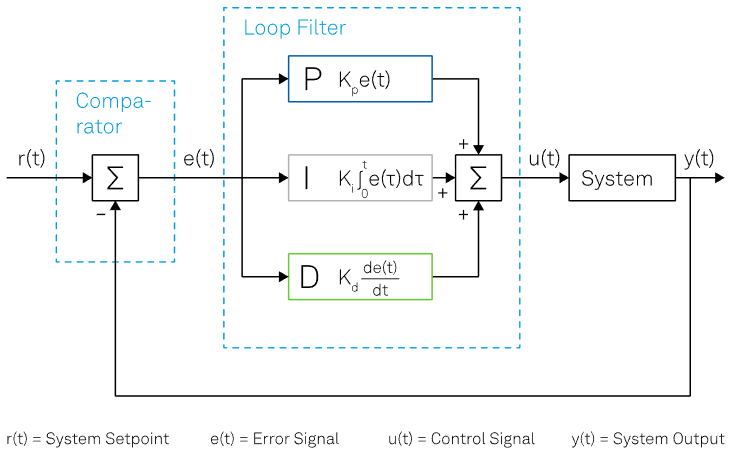
Figure 1. Schematic representation of a general PID control loop in its most general form. Image Credit: Zurich Instruments
Following this, the error signal is minimized by the loop filter and subsequently utilized to produce the control signal u(t) that drives the output of the system, initiating closed-loop operation.
These steps are performed repeatedly to minimize the error. As a result, apart from considering the current error, the consideration of its accumulation over time (represented by the integral) and its future tendency (represented by the derivative at time t) are also relevant. These are displayed in Figure 2.
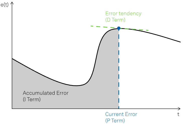
Figure 2. Example of error function with the highlighted contributions of the P, I and D terms. Image Credit: Zurich Instruments
The minimization of error is accomplished in the most general case by using the following three primary components of the PID controller loop filter: the proportional, integral, and derivative terms.
In its most general form, the complete control function may be written mathematically as the sum of the three individual contributions, as follows:
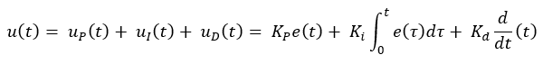
Where Kp, Ki, and Kd are the gain coefficients related to the proportional, integral, and derivative terms, respectively.
The Proportional Term
The proportional term is denoted by P and is based on the current error between the measured output of the system and the setpoint.
This term facilitates the output of the system being brought back to the setpoint by employing a correction that is proportional to the amplitude of the error. This results in a reduced rise time of the correction signal, as displayed in Figure 3.
The greater the error, the greater the correction applied by the proportional term, i.e., the greater the error with a fixed Kp, the greater uP(t).
Since the P term always requires a non-zero error to generate its output, it cannot nullify the error by itself. In steady-state system conditions, an equilibrium is reached, which includes a steady-state error.
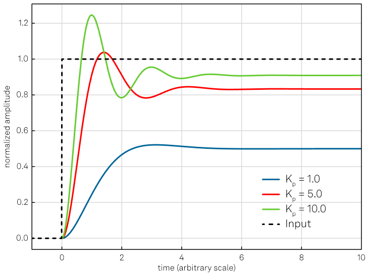
Figure 3. Effect of the proportional action. Increasing the Kp coefficient reduces the rise time, but the error never approaches zero. Additionally, a too high value of the proportional gain might lead to an oscillating output. Image Credit: Zurich Instruments
The Integral Term
The integral term is denoted by I and applies a correction that is proportional to the time integral of the error, i.e., the history of the error. For instance, if the error continues over time, the integral term continues to increase, leading to a greater correction being applied to the output of the system.
Unlike the proportional term, the integral term enables the controller to produce a non-zero control signal even under a zero-error condition at present. This allows the controller to bring the system to the exact required setpoint. Its effect is depicted in Figure 4.
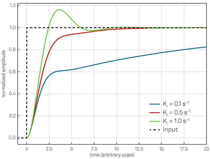
Figure 4. Effect of the integral action with constant Kp = 1. Increasing Ki, the response will be faster but also lead to larger oscillations and overshoot if the value increases too much (green curve). Image Credit: Zurich Instruments
Increasing the value of the integral gain coefficient leads to an increase in the contribution of the accumulated error over time to the control signal. This means that if a steady-state error exists, an integral term with a large gain coefficient will result in the control signal removing the error faster than a smaller integral term.
However, increasing the integral term too much may cause an oscillating output if excess error is accumulated. This results in the control signal overshooting and the creation of oscillations around the setpoint. This phenomenon is sometimes referred to as integral windup.2
The Derivative Term
The derivative term is denoted by D and provides control over the error tendency, i.e., its future behavior, through the application of a correction that is proportional to the time derivative of the error.
This enables the rate of change of the error to be reduced, which, in turn, enhances the stability and responsiveness of the control loop.
The goal is to anticipate the changes in the error signal: if the error exhibits an upward trend, the derivative action attempts to compensate before the error becomes significant (proportional action) or persists for some time (integral action).
In real-world implementations of PIDs, the derivative action may be omitted because of its high sensitivity to the quality of the input signal.
When the reference value rapidly changes, such as in the case of a very noisy control signal, the derivative of the error often becomes very large. This leads to the PID controller undergoing an abrupt change that can cause instabilities or oscillations in the control loop.
To enhance stability, prior low-pass filtering of the error signal is often used as a mitigation strategy; however, low-pass filtering and derivative control neutralize one another; thus, only a limited amount of filtering is possible.
If correctly calibrated and the system is sufficiently “tolerant,” the derivative action can provide a decisive contribution to the controller performance. Figure 5 illustrates the effect of the derivative term.
The effect of each term on the response of the system depends heavily on the system’s characteristics.
As a result, the weighting of the Kp, Ki, and Kd gains may be adjusted to fine-tune the performance of the control loop and to accomplish the desired accuracy and responsiveness.
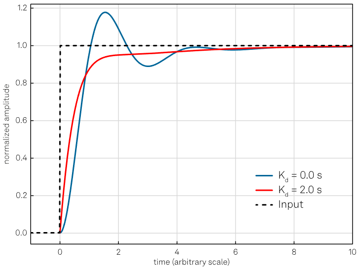
Figure 5. The purpose of the derivative action is to increase the damping of the system; however, too large values of Kd might make the system unstable or oscillatory, as described in the text. The curves are obtained keeping the proportional and integral gain constant (Kp = 4 and Ki = 1 s-1). Image Credit: Zurich Instruments
Some applications or simple systems may not require all three control terms provided by a PID controller. To operate the controller with only a subset of these terms, the unused terms can be set to zero, thus resulting in a PI, PD, P, or I controller.
For instance, due to their slow dynamics, a PI controller is commonly used in applications that prioritize steady-state error elimination and stability over fast response times.
One example of this is when controlling an oven’s temperature. In this scenario, a PI controller is typically employed to ensure precise temperature regulation and eliminate any steady-state offset, considering the oven’s relatively slow response characteristics.
Derivation of an Initial Set of Parameters (Tuning)
One of the key benefits of PID controllers is that they may be implemented without any prior knowledge or detailed model of the system.
Due to heuristic calibration procedures, coefficients may be calculated based only on simple experimental tests conducted directly on the process. However, the initial tuning of the PID parameters may still be a delicate task.
There are multiple well-established techniques to derive an initial set of coefficients, with many of these involving the measurement of open-loop parameters of the system.
As previously mentioned, open-loop refers to a system without any feedback control, i.e., an input signal is applied to the system, and the resulting output is only measured and not fed back to the input.
The input signal may be a step function, a sine wave, a ramp, or any other type of signal that is suitable for the system that is being controlled.
The output of the system is subsequently recorded as a function of time and may be analyzed to establish the response characteristics of the system, including its natural frequency, time constant, and damping ratio.
The general strategy to determine initial parameters typically involves the following three steps:
- Acquire the system’s open-loop response and measure some of the characteristic parameters, such as the oscillation period of the system output and the process delay.
- Determine coarse values of the gain coefficients Kp, Ki, and Kd using the measured parameters.
- Tune the PID gain coefficients to optimize for speed, noise, or robustness.
Some of the most popular methods to achieve coarse tuning are the Ziegler-Nichols method,3 the Cohen-Coon method,4 the relay method,5 and the Tyreus-Luyben method.6
A practical example of an initial tuning procedure is outlined in Table 1 and is constructed from the Ziegler-Nichols method.
Table 1. Step-by-step procedure for the Initial tuning of a PID controller, based on the Ziegler-Nichols method. Source: Zurich Instruments
| Set the P,I, and D gain to zero |
| ↓ |
| Increase the proportional (P) gain until the system starts to show consistent and stable oscillation. This value is known as the ultimate gain (Ku). |
| ↓ |
| Measure the period of the oscillation (Tu). |
| ↓ |
Depending on the desired type of control loop (P, PI or PID) set the gains to the following values:
| |
Kp |
Ki |
Kd |
| P controller |
0.5 Ku |
0 |
0 |
| PI controller |
0.45 Ku |
0.54 Ku / Tu |
0 |
| PID controller |
0.6 Ku |
1.2 Ku / Tu |
0.075 Ku Tu |
|
| ↓ |
| Test the response of the system and adjust the gains as necessary. If the response is too slow or sluggish, increase the P or I gain. If the response is too fast or oscillatory, decrease the P or I gain. If there is overshoot or ringing, increase the D gain. |
Principles of PID Controllers
References
- Maxwell James Clerk 1868. On governors, Proc. R. Soc. Lond.16270–283
- Y. Tian and D.P. Atherton. Analysis and Design of Reset Control Systems. Institution of Electrical Engineers, 2004.
- Ziegler, J. G., & Nichols, N. B. (1942). Optimum settings for automatic controllers. Transactions of the ASME, 64(6), 759-768.
- Cohen, H., & Coon, G. A. (1953). A linear operator approach to the analysis of closed-loop servomechanisms. Journal of the Franklin Institute, 256(6), 489-512
- Åström, K. J., & Hägglund, T. (1995). PID controllers: Theory, design, and tuning (2nd ed.). Instrument Society of America.
- Luyben, W. L. (1990). Plantwide control: Some practical considerations. Chemical Engineering Progress, 86(4), 49-53.

This information has been sourced, reviewed and adapted from materials provided by Zurich Instruments.
For more information on this source, please visit Zurich Instruments.