Assessing wastewater for metallic contamination is critical for safeguarding public health and the environment from the adverse effects of inadequately treated municipal wastewaters and specific industrial discharges.

Image Credit: Andromeda stock/Shutterstock.com
However, the regulatory frameworks for wastewater differ significantly between countries. In the United States, the Environmental Protection Agency (EPA), in conjunction with state agencies, negotiates discharge permits under the National Pollutant Discharge Elimination System (NPDES).
This process takes into account federal guidelines for industrial categories (40 CFR, Parts 405-471) and the ecological sensitivity of the receiving water bodies at each site.1
The treatment of wastewater within the EU is governed by the Urban Wastewater Treatment Directive (UWTD) and the Integrated Pollution and Control (IPC) Directive, both operating under the EU Water Framework Directive (WFD).
German wastewater regulations, known as the Abwasserverordnung (AbwV), integrate various EU directives pertaining to discharge limits for pollutants, aiming to reduce environmental pollution.
Unlike the wastewater discharge regulations enforced by the Clean Water Act (CWA) in the US, the German AbwV does not distinguish between direct and indirect discharges. Both categories must comply with the requirements set for individual industries or communal wastewater.
Consequently, wastewater requires the measurement of a diverse range of metals at varying concentrations, within different water matrices.
Several inorganic analytical methods are available for determining the elemental composition of wastewater. These include atomic absorption spectroscopy (AAS), inductively coupled plasma optical emission spectroscopy (ICP-OES), and ICP mass spectrometry (ICP-MS).
The most appropriate technique for each specific requirement can be chosen based on the number of elements and samples involved. While ICP-MS excels in highly precise trace detection, it is not well-suited for accurately and precisely determining mineral content at levels of 200 mg/L.
Standard ICP-OES instruments generally provide superior performance for assessing mineral and pollutant concentrations, but frequently lack the sensitivity needed to reliably detect toxic trace metals. The application of ICP-OES is described in various standard procedures, such as US-EPA Method 200.7 or ISO 11885.2-3
The US EPA developed Method 200.7 specifically for the determination of metals and trace elements in waters and waste materials using ICP-OES. This method is applicable to a variety of sample types, but it is extensively employed for wastewater applications.
The method incorporates a quality control program to ensure the proper operation of both the instrument and the analytical methodology during the analysis of wastewater samples.
In this study, the PlasmaQuant 9200 Elite ICP-OES - recognized for its high sensitivity, broad linear dynamic range, and exceptional spectral resolution - was evaluated for wastewater analysis.
The approach presented here details the analysis of pollutants and trace elements in wastewater using a standard ICP-OES configuration. The suitability of this methodology was validated through a quality control program aligned with Method 200.7.
This included: the analysis of several certified reference materials, participation in a national proficiency testing program for external quality assurance, assessment of spike recoveries in challenging matrices, and monitoring of the system's long-term stability.
Materials and Methods
Sample Preparation
All laboratory equipment was cleaned with deionized (DI) water from a PURELAB system (18.2 MΩ cm, ELGA LabWater, High Wycombe, England).
Single- and multi-element working standards were prepared by serial volume/volume dilution in polypropylene tubes from stock solutions (Merck, Sigma-Aldrich, CPAChem, Inorganic Ventures) using 1 % (v/v) sub-boiled distilled HNO3.
All samples (unless already stabilized) and blank solutions were acidified with HNO3 to yield a final acid concentration of 1 % (v/v). Yttrium (Y) was introduced online to all blanks, standards, and samples as an internal standard.
This study also incorporated various water types (surface and ground water) and wastewater samples, along with reference materials used for validating the developed method, as summarized in Table 1.
Three of the analyzed wastewater samples were part of a national round robin test (RRT) (“59th National Round Robin Test- Elements in Wastewater - 03/21” from the Staatliche sBetriebsgesellschaft für Umwelt und Landwirtschaft Sachsen(BfUL), Germany).
All samples were acidified with sub-boiled HNO3 to achieve a final acid concentration of 1 % (v/v), with the exception of the RRT samples.
Sample preparation for the RRT samples was conducted in accordance with EPA Method 3015A (SW-846) and DIN EN ISO 15587-2, which necessitate a microwave-assisted acid digestion step.
Consequently, a 25.0 (± 0.1) mL aliquot of the sample and 6.25 (± 0.10) mL of sub-boiled HNO3 were added to a digestion vessel (PM60). The mixture was gently swirled and allowed to stand for at least 15 minutes before the vessel was sealed.
Subsequent heating (20 minutes at 200 °C) was performed in a speedwave XPERT microwave digestion system. Afterward, the vessels were cooled to room temperature (RT) to prevent foaming and splashing. The resulting solutions were transferred to a graduated polypropylene tube and diluted to 50 mL with DI water.
In the case of Mercury (Hg), the sample preparation for the RRT samples was modified to fully comply with DIN EN ISO 12846: 2012-08 (E12). The samples arrived already stabilized (1 mL concentrated HCl per 100 mL) and were stored exclusively in glass containers throughout the entire procedure.
For preparation, 25 (± 0.1) mL of each sample were added to a 50 mL glass vial, combined with 0.5 mL of a 1:1 solution of potassium bromide (c (KBr) = 0.2 mol/L) and potassium bromate (c (KBrO3) = 0.033 mol/L), and incubated (24 hours at RT).
Following incubation, 10 µL of hydroxylammonium chloride (NH2OH x HCl, 120 g/L) and 0.5 mL of sub-boiled HCl were added to the reaction mixture, which was then analyzed immediately. Blank and standard solutions were prepared accordingly.
The determination of Hg is based on a cold vapor technique. The reducing agent comprised 3 g of sodium borohydride (NaBH4) and 1 g of sodium hydroxide (NaOH) dissolved in one liter of DI water, yielding concentrations of 0.3 % (m/v) and 0.1 % (m/v), respectively. Samples were diluted tenfold with 5 % (v/v) sub-boiled HCl and analyzed.
Table 1. List of samples and reference materials being analyzed. Source: Analytik Jena
| Sample |
Supplier |
| Certified wastewater-Trace metals solution A (CWW-TM-A) |
High Purity Standards |
| Certified wastewater-Trace metals solution B (CWW-TM-B) |
High Purity Standards |
| Certified wastewater-Trace metals solution C (CWW-TM-C) |
High Purity Standards |
| Certified wastewater-Trace metals solution D(CWW-TM-D) |
High Purity Standards |
| ERM-CA713 Wastewater (trace elements) |
Sigma-Aldrich |
| RRT wastewater sample A |
BfUL |
| RRT wastewater sample B |
BfUL |
| RRT wastewater sample C |
BfUL |
| Industrial effluent – Inlet |
Automobile industry |
| Industrial effluent – Inlet |
Galvanic industry |
Calibration
For each element, calibration levels were chosen based on expected concentration ranges. A minimum of three calibration standards were employed for each element, as seen in Table 2. Figure 1 depicts selected calibration curves.
Table 2. Concentration of calibration standards. Source: Analytik Jena
| Standard |
Concentration [mg/L] |
Ag, Al, As, B, Ba, Be,
Bi, Cd, Co, Cr, Cu, Fe,
Li, Mn, Ni, Pb, Se, Sr,
Te, Tl, V, Zn |
Mg, P,
Si |
Ca, K,
Na |
Mo, Sb,
Sn, Ti |
Hg |
| Calibration 0 |
0 |
0 |
0 |
0 |
0 |
| Standard 1 |
0.01 |
0.01 |
- |
- |
- |
| Standard 2 |
0.1 |
0.1 |
0.1 |
- |
- |
| Standard 3 |
1.0 |
1.0 |
1.0 |
- |
- |
| Standard 4 |
- |
10.0 |
10.0 |
- |
- |
| Standard 5 |
- |
- |
100 |
- |
- |
| Standard 6 |
- |
- |
- |
0.01 |
- |
| Standard 7 |
- |
- |
- |
0.1 |
- |
| Standard 8 |
- |
- |
- |
1.0 |
- |
| Standard 9 |
- |
- |
- |
- |
0.005 |
| Standard 10 |
- |
- |
- |
- |
0.01 |
| Standard 11 |
- |
- |
- |
- |
0.025 |
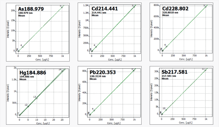
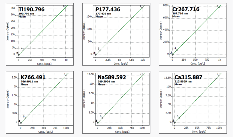
Figure 1. Selected calibration functions. Image Credit: Analytik Jena
Instrument Settings
The analysis was performed on a PlasmaQuant 9200 Elite ICP-OES. The sample introduction components and instrumental parameters were selected to achieve a high level of sensitivity for trace elements in matrices that might contain high salt concentrations.
A Teledyne CETAC ASX-560 Autosampler was used in conjunction with this instrument. An internal standard mixing kit was also employed to introduce a 10 mg/L yttrium internal standard solution online, resulting in an approximate final concentration of 1 mg/L. Table 3 provides a summary of individual settings and components.
Table 3. Instrument settings. Source: Analytik Jena
| Parameter |
Specification |
| Plasma power |
1250 W |
| Plasma gas flow |
8.5 L/min |
| Auxiliary gas flow |
0.4 L/min |
| Nebulizer gas flow |
0.6 L/min |
| Nebulizer |
Concentric, SeaSpray, 2.0 mL/min, Borosilicate |
| Spray chamber |
Cyclonic spray Chamber, 50 mL, Borosilicate |
| Outer tube/Inner tube |
Quartz/Quartz |
| Injector |
Quartz, ID: 2 mm |
| Sample tubing |
PVC (red/red) |
| Internal standard tubing |
PVC (green/orange) |
| Pump rate |
1.00 mL/min |
| Fast pump |
4.0 mL/min |
| Measuring delay/Rinse time |
45 s/15 s |
| Torch position |
0 mm |
Method and Evaluation Parameters
Table 4. Method parameters. Source: Analytik Jena
| Element |
Line |
Plasma View |
Integration |
Read Time |
Evaluation |
| [nm] |
|
|
[s] |
Pixel |
Baseline Fit |
Poly. Deg. |
| Y |
371.030 |
axial/radial |
Peak |
1/2 |
3 |
ABC1 |
auto |
| Ag |
328.068 |
axial |
Peak |
1 |
3 |
ABC |
auto |
| Al |
394.401 |
axial |
Peak |
3 |
3 |
ABC |
auto |
| As |
188.979 |
axial |
Peak |
10 |
3 |
ABC |
auto |
| B |
249.773 |
axial |
Peak |
3 |
3 |
ABC |
auto |
| Ba |
455.403 |
radial |
Peak |
1 |
3 |
ABC |
auto |
| Be |
313.107 |
axial |
Peak |
2 |
3 |
ABC |
auto |
| Bi |
223.061 |
axial |
Peak |
10 |
3 |
ABC |
auto |
| Ca |
315.887 |
radial |
Peak |
1 |
3 |
ABC |
auto |
| Cd |
214.441 |
axial |
Peak |
3 |
3 |
ABC |
auto |
| Co |
228.615 |
axial |
Peak |
3 |
3 |
ABC |
auto |
| Cr |
267.716 |
axial |
Peak |
1 |
3 |
ABC |
auto |
| Cu |
327.396 |
axial |
Peak |
3 |
3 |
ABC |
auto |
| Fe |
259.940 |
axial |
Peak |
1 |
3 |
ABC |
auto |
| Hg |
184.886 |
axial |
Peak |
10 |
3 |
ABC |
auto |
| K |
766.491 |
radial |
Peak |
1 |
3 |
ABC |
auto |
| Li |
670.791 |
radial |
Peak |
3 |
3 |
ABC |
auto |
| Mg |
285.213 |
radial |
Peak |
1 |
3 |
ABC |
auto |
| Mn |
257.610 |
axial |
Peak |
1 |
3 |
ABC |
auto |
| Mo |
202.030 |
axial |
Peak |
3 |
3 |
ABC |
auto |
| Na |
589.592 |
radial |
Peak |
1 |
3 |
ABC |
auto |
| Ni |
231.604 |
axial |
Peak |
3 |
3 |
ABC |
auto |
| P |
177.436 |
axial |
Peak |
3 |
3 |
ABC |
auto |
| Pb |
220.353 |
axial |
Peak |
10 |
3 |
ABC |
auto |
| Sb |
217.581 |
axial |
Peak |
10 |
3 |
ABC |
auto |
| Se |
196.028 |
axial |
Peak |
10 |
3 |
ABC |
auto |
| Si |
251.611 |
radial |
Peak |
1 |
3 |
ABC |
auto |
| Sn |
189.927 |
axial |
Peak |
3 |
3 |
ABC |
auto |
| Sr |
407.771 |
radial |
Peak |
1 |
3 |
ABC |
auto |
| Te |
214.281 |
axial |
Peak |
10 |
3 |
ABC |
auto |
| Ti |
334.941 |
axial |
Peak |
3 |
3 |
ABC |
auto |
| Tl |
190.796 |
axial |
Peak |
10 |
3 |
ABC |
auto |
| V |
292.401 |
axial |
Peak |
3 |
3 |
ABC |
auto |
| Zn |
206.200 |
axial |
Peak |
1 |
3 |
ABC |
auto |
1 ... Automated Baseline Correction
Results and Discussion
EPA method 200.7 mandates a formal quality control (QC) program. This program involves, at a minimum, the initial demonstration of laboratory capability, and the ongoing analysis of blanks and other laboratory standards to ensure instrument performance.
The first demonstration of laboratory capability includes the determination of method detection limits (MDLs) and linear dynamic range (LDR), periodical checks of blank solutions, instrument performance checks (IPC), and spectral interference checks (SIC). Additionally, the accuracy and long-term stability of the method must be evaluated.
Linear Dynamic Range and Method Detection Limits
According to Method 200.7, the LDR is defined as the upper limit at which values are recovered within 10 % of the actual concentration when determined against the calibration curve used for analysis.
The MDLs are derived from seven measurements of a blank solution that has been spiked at a concentration two to three times the instrument detection limit. The standard deviation of these seven measurements is then multiplied by 3.14 (at a 99 % confidence level) to ascertain the MDL.
Table 5 presents the method-specific LDRs and MDLs.
Table 5. Method detection limits (MDL) and upper limit of the linear dynamic range (LDR) for the employed analytical lines. Source: Analytik Jena
| Element |
Line
[nm] |
Plasma
View |
MDL
[μg/L] |
LDR
[mg/L] |
| Ag |
328.068 |
axial |
0.14 |
20* |
| Al |
394.401 |
axial |
0.55 |
100* |
| As |
188.979 |
axial |
0.35 |
100* |
| B |
249.773 |
axial |
0.20 |
100* |
| Ba |
455.403 |
radial |
0.06 |
10 |
| Be |
313.107 |
axial |
0.01 |
5 |
| Bi |
223.061 |
axial |
0.35 |
100* |
| Ca |
315.887 |
radial |
1.38 |
250 |
| Cd |
214.441 |
axial |
0.04 |
10 |
| Co |
228.615 |
axial |
0.12 |
50 |
| Cr |
267.716 |
axial |
0.10 |
50 |
| Cu |
327.396 |
axial |
0.11 |
100* |
| Fe |
259.940 |
axial |
0.08 |
25 |
| Hg |
184.886 |
axial |
0.14 |
10* |
| K |
766.491 |
radial |
22.0 |
200 |
| Li |
670.791 |
radial |
0.23 |
25 |
| Mg |
285.213 |
radial |
0.25 |
100* |
| Mn |
257.610 |
axial |
0.02 |
10 |
| Mo |
202.030 |
axial |
0.13 |
100* |
| Na |
589.592 |
radial |
4.08 |
250 |
| Ni |
231.604 |
axial |
0.12 |
20* |
| P |
177.436 |
axial |
1.25 |
100 |
| Pb |
220.353 |
axial |
0.35 |
20* |
| Sb |
217.581 |
axial |
0.40 |
100* |
| Se |
196.028 |
axial |
1.25 |
100* |
| Si |
251.611 |
radial |
2.90 |
100 |
| Sn |
189.927 |
axial |
0.25 |
100* |
| Sr |
407.771 |
radial |
0.04 |
5 |
| Te |
214.281 |
axial |
0.88 |
100* |
| Ti |
334.941 |
axial |
0.02 |
20* |
| Tl |
190.796 |
axial |
0.45 |
100* |
| V |
292.401 |
axial |
0.04 |
50 |
| Zn |
206.200 |
axial |
0.08 |
10 |
* Upper limit of test: even higher concentrations are possible by fulfilling the 90 % recovery criteria
Laboratory Reagent Blank (LRB) and Laboratory Fortified Blank (LFB)
Method 200.7 requires regular measurements of distinct blank solutions. One of these is the laboratory reagent blank (LRB), which is processed identically to samples, incorporating all reagents in the same volumes.
It should be analyzed with each batch of 20 or fewer samples (of the same matrix) to detect potential contamination from the laboratory environment and should not exceed 10 % of the determined analyte levels, or be smaller than 2.2 times the MDL.
The other blank is the laboratory fortified blank (LFB), which is prepared by spiking an aliquot of the LRB with a suitable analyte concentration. The LFB must also undergo the complete sample preparation process and should be analyzed with each batch of samples.
The accuracy, calculated as percent recovery, must fall within a ± 15 % control limit. All LRBs and LFBs were prepared and analyzed in compliance with Method 200.7 and met all stipulated criteria.
Quality Control Sample, Instrument Performance Check, and Stability
Immediately after calibration, two different QC samples must be analyzed to confirm the quality of calibration standards and instrument performance. These include the quality control sample (QCS) and the initial performance check (IPC) solution.
The IPC should originate from the same source, while the QCS must be prepared from a different stock solution. The recovery for both standards must be within ± 5 % of the specified value.
The specific standards were spiked at 0.01 mg/L (Hg), 0.5 mg/L (for most elements), 5 mg/L (for magnesium (Mg), phosphorous (P), and silicon (Si)), and 50 mg/L (for calcium (Ca), potassium (K), and sodium (Na)), respectively. Figure 2 indicates that all elements fulfilled the criterion.
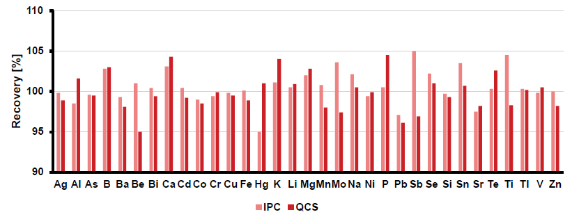
Figure 2. Recoveries for the initial IPC (pink) and QCS (red). Image Credit: Analytik Jena
Furthermore, the quality program mandates the continuous measurement (after every 10 analyses and at the conclusion of the run) of the IPC throughout the entire analytical sequence.
The ongoing IPC results consistently remained within the acceptable range of 90–110 % of the known value, as shown in Figure 3. Figure 4 illustrates the behavior of the internal standard yttrium in both axial and radial observational views.
Relative standard deviations below 1.55 % signify highly stable instrumentation performance over the 14-hour measurement period.
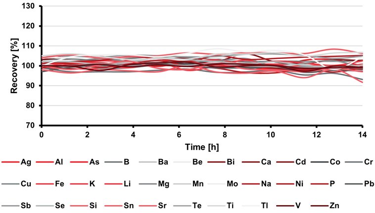
Figure 3. Percentage recoveries in the IPC solutions throughout a 14-hour sequence. RSD values were below 1.65 % for all elements. Image Credit: Analytik Jena
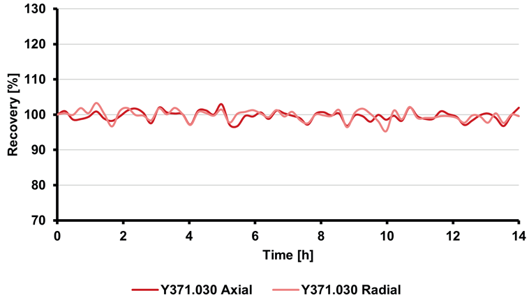
Figure 4. Percentage recoveries of the internal standard (yttrium) throughout a 14-hour sequence. RSD values were below 1.55 % for both observational views. Image Credit: Analytik Jena
Spectral Interference Check
As a component of the QC program, a spectral interference check (SIC) solution must be tested periodically to verify the interelemental spectral correction routine.
For instruments that do not leverage interelement corrections (IEC), SIC solutions (containing similar concentrations of major sample components, e.g., ≥ 10 mg/L) can be used to confirm the absence of spectral interferences at the selected analytical wavelengths.
Given that the PlasmaQuant 9200 Elite uses a high-resolution optical system (2 pm @ 200 nm), access to the most common elemental lines is ensured, thereby rendering IEC tools obsolete. Nevertheless, an SIC solution containing 200 mg/L aluminum (Al) and 300 mg/L iron (Fe) was analyzed and seen to demonstrate no significant interferences at the chosen wavelengths.
Assessing Analyte Recovery
The chemical nature of the sample matrix can influence analyte recovery, meaning that Method 200.7 requires spiking experiments in at least 10 % of routine samples prior to sample preparation.
The recovery of the spiked analyte concentration must be within ±30 % of the concentration added to the sample. To address this, high-solid wastewater samples from the automobile and galvanic industries were spiked before sample preparation with 0.5 mg/L of the target elements.
Figure 5 presents the analyte recoveries, all of which fell within a ±20 % range, demonstrating the applicability of the analytical method.
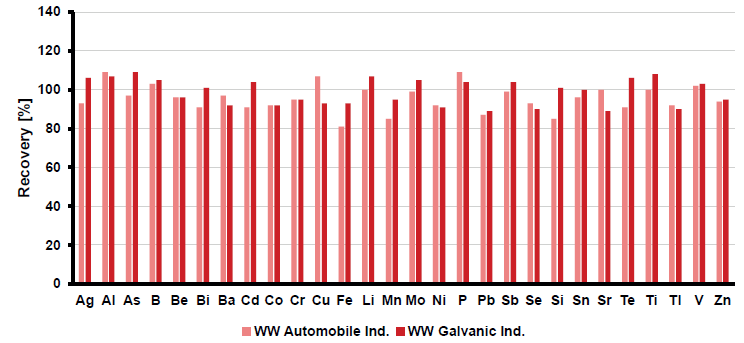
Figure 5. Spike recoveries of 0.5 mg/L in wastewater samples originating from automobile (pink) and galvanic industry (red). Analytes were spiked before microwave digestion following EPA Method 3015A (SW-846) and DIN EN ISO 15587-2. Image Credit: Analytik Jena
Moreover, reference materials can be analyzed to show the validity of a method. As a result, four wastewater reference materials were analyzed. Table 6 lists the certified values and recovery rates for the tested reference materials.
All recoveries were within ±10 % of the certified value. Moreover, a wastewater reference material containing low concentrations - close to or under the legal limits of important drinking water regulations - of arsenic (As), mercury (Hg), and selenium (Se) was analyzed.
The recovery rates for these elements were within ±14 %, indicating the method's applicability for critical elements, such as As and Hg, even at lower concentration ranges that approach or fall below legal limits when using a standard sample introduction kit.
Table 6. Quantitative results for several certified reference materials (CRMs). Source: Analytik Jena
| Element |
CWW-TM-A |
CWW-TM-B |
CWW-TM-C |
CWW-TM-D |
Certified
[μg/L] |
Recovery
[%] |
Certified
[μg/L] |
Recovery
[%] |
Certified
[μg/L] |
Recovery
[%] |
Certified
[μg/L] |
Recovery
[%] |
| Ag |
10 |
97 |
50 |
96 |
150 |
99 |
250 |
98 |
| Al |
50 |
95 |
200 |
99 |
500 |
99 |
1000 |
99 |
| As |
10 |
95 |
50 |
97 |
150 |
97 |
250 |
96 |
| B |
50 |
100 |
200 |
101 |
500 |
102 |
1000 |
102 |
| Baradial |
50 |
99 |
200 |
98 |
500 |
99 |
1000 |
98 |
| Be |
10 |
95 |
50 |
97 |
150 |
98 |
250 |
98 |
| Cd |
10 |
98 |
50 |
97 |
150 |
97 |
250 |
98 |
| Co |
50 |
97 |
200 |
98 |
500 |
98 |
1000 |
98 |
| Cr |
50 |
98 |
200 |
100 |
500 |
100 |
1000 |
97 |
| Cu |
50 |
98 |
200 |
100 |
500 |
101 |
1000 |
101 |
| Fe |
50 |
98 |
200 |
100 |
500 |
99 |
1000 |
97 |
| Mn |
50 |
99 |
200 |
100 |
500 |
98 |
1000 |
98 |
| Mo |
50 |
97 |
200 |
98 |
500 |
98 |
1000 |
97 |
| Ni |
50 |
97 |
200 |
100 |
500 |
99 |
1000 |
98 |
| Pb |
50 |
99 |
200 |
100 |
500 |
97 |
1000 |
99 |
| Sb |
10 |
90 |
50 |
90 |
150 |
91 |
250 |
90 |
| Se |
10 |
94 |
50 |
100 |
150 |
100 |
250 |
101 |
| Srradial |
50 |
98 |
200 |
101 |
500 |
101 |
1000 |
99 |
| Tl |
10 |
94 |
50 |
100 |
150 |
102 |
250 |
99 |
| V |
50 |
98 |
200 |
101 |
500 |
100 |
1000 |
100 |
| Zn |
50 |
99 |
200 |
98 |
500 |
99 |
1000 |
99 |
Table 7. Quantitative results for certified reference material WW CA 713. Source: Analytik Jena
| Element |
WW CA 713 |
| Certified [μg/L] |
Recovery [%] |
| As |
10.8 |
107 |
| Cd |
5.09 |
93 |
| Cr |
20.9 |
97 |
| Cu |
101 |
106 |
| Fe |
445 |
95 |
| Hg |
1.84 |
105 |
| Mn |
95 |
96 |
| Ni |
50.3 |
96 |
| Pb |
49.7 |
92 |
| Se |
4.9 |
86 |
| Zn |
78 |
100 |
External Quality Control: Round Robin Test
A round robin (or proficiency) test (RRT) is a method of external quality assurance for various measurement procedures.
Fundamentally, identical samples are analyzed using the same or different procedures in multiple laboratories. Comparing the results allows for statements to be made about general measurement accuracy or the measurement quality of the participating laboratory.
To demonstrate the performance of the PlasmaQuant 9200 and the applicability of the analytical method, the application laboratory at Analytik Jena's headquarters participated in a national round robin test.
This test involved the analysis of three wastewater samples. Sample preparation was conducted as described in the “Samples and Reagents” section. The organizer of the RRT specified the approved analytical methods and the corresponding regulations for sample preparation.
Table 8. Quantitative results for round robin test samples. Source: Analytik Jena
| Element |
Wasterwater Sample A |
Wasterwater Sample B |
Wasterwater Sample C |
Assigned
[μg/L] |
Measured
[μg/L] |
z-scorea |
Assigned
[μg/L] |
Measured
[μg/L] |
z-score |
Assigned
[μg/L] |
Measured
[μg/L] |
z-score |
| Al |
1664.029 |
1640 |
-0.2 |
296.473 |
298 |
0.1 |
1256.799 |
1258 |
0.0 |
| As |
34.785 |
34.3 |
-0.1 |
86.134 |
81.4 |
-0.8 |
175.277 |
166.2 |
-0.9 |
| Cd |
2.741 |
2.69 |
-0.2 |
0.824 |
0.870 |
0.4 |
6.011 |
5.34 |
-1.4 |
| Cr |
385.734 |
415 |
1.6 |
96.992 |
92.3 |
-1.0 |
174.162 |
173 |
-0.1 |
| Cu |
258.785 |
257 |
-0.1 |
375.709 |
371 |
-0.2 |
86.059 |
84.8 |
-0.2 |
| Fe |
180.552 |
190 |
0.6 |
362.468 |
355 |
-0.7 |
850.259 |
841 |
-0.6 |
| Hgb |
0.371 |
0.299 |
-0.9 |
1.017 |
0.852 |
-0.7 |
1.522 |
1.28 |
-0.7 |
| Ni |
397.862 |
410 |
0.5 |
120.354 |
115 |
-0.8 |
199.558 |
188 |
-1.0 |
| Pb |
54.707 |
55.8 |
0.2 |
131.381 |
122 |
-0.7 |
76.425 |
71.6 |
-1.0 |
| Zn |
96.561 |
94.8 |
-0.2 |
167.401 |
156 |
-0.8 |
361.720 |
343 |
-0.8 |
a Calculation of z-score was performed in accordance to DIN 38402-45:2014-06
b Determined by using cold vapor ICP-OES
The concentration of Hg in the RRT samples was determined using cold vapor ICP-OES. To achieve this, the PlasmaQuant 9200 Elite was equipped with the hydride generation system HS PQ Pro (see Figure 6). With the addition of this system, the unique sensitivity of the HR-Array ICP-OES PlasmaQuant 9200 Elite was further improved, reaching detection limits below 10 ng/L for Hg.
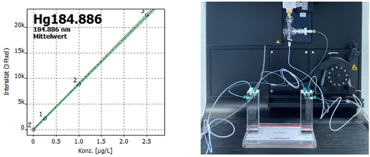
Figure 6. Calibration curve for the analytical line of Hg at 184 nm using cold vapor ICP-OES (left). On the right, the HS PQ Pro is shown in the sample chamber of the PlasmaQuant 9200 Elite. Image Credit: Analytik Jena
Summary
The method presented here describes the use of a high-resolution ICP-OES in a standard configuration, fully adhering to the requirements of EPA Method 200.7 for a wide range of diverse wastewater samples.
It was demonstrated that the PlasmaQuant 9200 Elite successfully meets the stringent quality control requirements of the method by providing excellent sensitivity, accuracy, and long-term stability.
Furthermore, the instrument's performance and the applicability of the analytical method were successfully confirmed by passing a national round robin test.
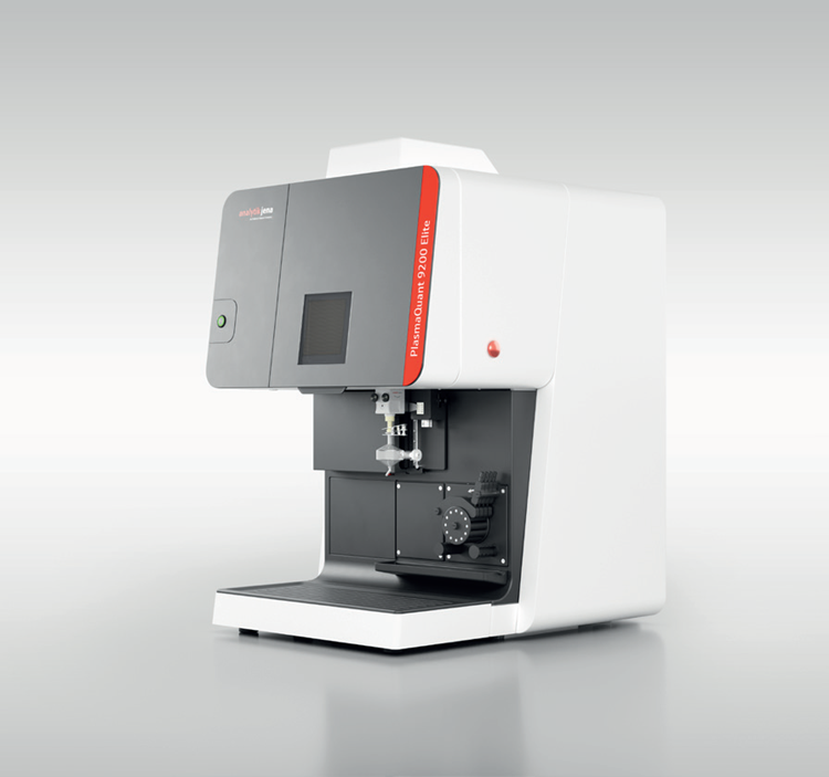
Figure 7. PlasmaQuant 9200 Elite. Image Credit: Analytik Jena
The primary challenge in this application lies in analyzing elements across a broad concentration spectrum (from low µg/L to high mg/L) in a single run. Trace elements (e.g., As, Hg) need to be analyzed alongside highly concentrated minerals (e.g., Mg, Na) and pollutants (e.g., Al, Fe), a task successfully managed by the DualView Plus feature of the PlasmaQuant 9200 Elite.
Beyond the standard radial and axial plasma observation modes, it offers axial plus and radial plus views that attenuate the signal in the respective observation mode. The method described here leverages radial plasma observation for measuring high mineral levels, coupled with axial view for trace levels of toxic elements in a single measurement run. This eliminates the need for multiple dilutions to cover the entire concentration range.
The method validation encompassed accuracy determination on CRMs and several spiked wastewater samples, illustrating the suitability of the PlasmaQuant 9200 Elite ICP-OES system to meet wastewater and drinking water directives, such as the Safe Drinking Water Act, the European Drinking Water Directive, or the German drinking water ordinance.
A typical problem with ICP-OES instrumentation is insufficient sensitivity to comply with regulations for trace element detection. In this regard, the PlasmaQuant 9200 Elite offers high sensitivity, attributed to numerous technical features.
The high-efficiency generator produces a robust plasma, delivering strong and consistent signal intensity with minimal argon consumption, even for wastewater samples with high salt content.
Additionally, the spectral resolution of 2 pm @ 200 nm (Figure 8) makes the use of complex correction algorithms, such as inter-element correction, unnecessary. This enables reliable and interference-free quantification of trace elements by providing access to the most sensitive emission lines and high-definition peak shapes with enhanced sensitivity.
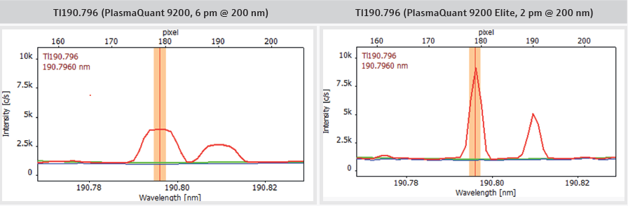
Figure 8. Comparison of PlasmaQuant 9200 (6 pm @ 200 nm) and PlasmaQuant 9200 Elite (2 pm @ 200 nm) illustrating the application advantage of high-resolution spectra (red: IPC, blue: blank, green: baseline correction (ABC)). Image Credit: Analytik Jena
The proposed setup fulfills all criteria for water and wastewater quality monitoring. The employment of the PlasmaQuant 9200 Elite allows water laboratories to conduct their entire elemental screening on a single instrument by using a standard sample introduction kit, leading to cost savings, reduced lab space requirements, and efficient use of time and labor.
Performance can be further augmented by incorporating a hydride system to lower the method detection limits for mercury and hydride-forming elements into the ng/L range.
Recommended Device Configuration
Table 9. Overview of devices, accessories, and consumables. Source: Analytik Jena
| Article |
Article number |
Description |
| PlasmaQuant 9200 Elite |
818-09201-2 |
High resolution ICP-OES |
| STANDARD KIT for PlasmaQuant 9x00 series |
810-88006-0 |
Sample introduction kit for aqueous samples |
Concentric nebulizer 2 mL/min
Borosilicate glass, for high salt content |
418-13-410-609 |
Nebulizer for improved robustness and stability |
| Teledyne Cetac ASX-560 |
810-88015-0 |
Autosampler with integrated rinse function |
References
- 40 CFR, Parts 405-471, U.S. Code of Federal Regulations
- EPA Method 200.7, “Determination of Metals and Trace Metals in Water and Wastes by Inductively Coupled Plasma Atomic Emission Spectrometry”, Rev. 4.4
- ISO. ISO 11885:2007. “Water quality - Determination of selected elements by inductively coupled plasma optical emission spectrometry (ICP-OES)”. Available at: https://www.iso.org/standard/36250.html.

This information has been sourced, reviewed and adapted from materials provided by Analytik Jena.
For more information on this source, please visit Analytik Jena.