Elemental and particle count identification answers two of the most critical questions in oil analysis: “How many?” and “Where is it coming from?” These two measurements are the most important in machine condition monitoring applications.
Using current technologies, the particle count is usually a pre-screen for performing root cause analysis using XRF, EDX/SEM, and in some cases, ferrography. However, these techniques have been shown to be labor intensive, time consuming, and expensive.
Although other routine elemental tests are also used, they are particle size sensitive toward the small fines, and they do not provide the best solution for detecting normal to abnormal wear transition.
Typically, machine condition through oil analysis is monitored by measuring the size, number, and elemental composition of wear particles that are produced at the extremities of lubricated machine components. The quantity and size of these wear particles has a direct correlation to a benign vs an abnormal wear state, as shown in Figure 1.
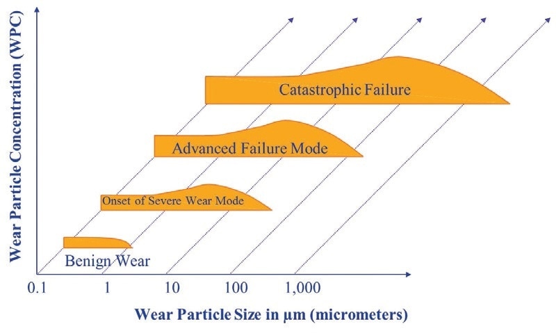
Figure 1. Progressions to Failure
It must be noted that a benign wear state in one type of machine will differ from another. In such cases, the size and quantity of the normal benign wear are governed by the type of wear mechanism along with the load, contact area, lubricant condition, and speed.
This makes limit and alarm settings difficult compared to cleanliness control applications, where the level of overall contamination must meet a maximum threshold. This threshold is a fixed limit (usually specified by the OEM) and it is often small enough to be measured by light blocking laser particle counters. Particle count standards such as NAS1638 and ISO 4406 were specifically developed for these types of applications.
Filtration and other loss mechanisms in lubricant systems, which readily generate wear, also play an important role in the overall particle picture. Filters are primarily responsible for the condition of dynamic equilibrium for a given particle size [1] , and set alarms and baselines for large particles.
Very fine particles do not work well in this model as they are diluted into the system, making baseline measurements impossible. Fewer small particles are created by the transition from a normal benign wear mode to an abnormal wear mode. This is because the forces acting on the shear mixed layer are now greater, and fine rubbing wear substitutes for much larger wear particles produced from under the shear mixed layer [2].
Based on the wear mode, different types of wear particles are produced by machines. These are explained in more detail in the Wear Particle Atlas [3].
Existing Machine Failure Measurement Techniques
Particle Count
Particle count indicates the severity of a wear situation, and the transition from small to large particles can be detected easily. One of the following techniques is usually used to perform particle count: laser light blockage, pore blockage, or direct imaging.
Laser light blocking suffers from the ability to see through dark sooted samples and from coincidence effects (particle overlap). As a result, this process is limited to clean translucent fluids employed in the contamination control industry, where there is minimal internal machine contact.
Direct imaging counters the coincidence effect by processing particles across a larger area using a CCD sensor. The sample is illuminated by a pulsed laser diode which can increase light throughput and overcome dark sooted samples, to approximately 2% prior to dilution.
Conventional pore blockage devices are similar to optical particle counters as they saturate at relatively low levels and are not ideal to accurately quantify heavily contaminated machine wear samples. However, these devices are able to process oils containing water or soot as these contaminants can easily pass through the pores without increasing the signal output. This is the primary advantage of pore blockage methods over direct imaging and light blocking methods.
LNF Compared to Traditional Ferrography
Atomic Emission Spectroscopy
Traditionally, elemental identification of wear particles has been carried out using atomic emission spectroscopy by either Inductively Coupled Plasma (ICP) or Rotating Disc Electrode (RDE). However, when it comes to detecting large particles, these methods are limited.
As a result, other complementary methods have been developed to help to increase the large particle detection capability of atomic emission. These methods include acid digestion and Rotrode Filter Spectroscopy (RFS). However, the additional methods take a long time and require a lot of special sample preparation and, in the case of acid digestion, hazardous chemicals are employed.
X-ray Fluorescence (XRF)
X-ray Fluorescence (XRF) is a common method that measures individual chemical elements in used oil samples. Generally, samples are analyzed by taking an x-ray of a small amount of oil sample (1 - 2 ml) in a cup. Similar to atomic emission techniques, the large particles related to abnormal failure modes are not suited to the analysis technique using a cup. This is because the focused XRF beam spot fails to statistically represent the large particle distribution in just 1 - 2 ml of oil.
While these results correlate well with ICP and RDE, the overall elemental signal is much lower. This is anticipated depending on the small XRF beam spot compared to the overall oil volume being analyzed.
When this technique is used, interference from small sub micron carbonaceous soot particles also creates problems for heavily sooted diesel engine oil samples. These samples need some form of baseline calibration to compensate the soot interference.
Better sensitivity can be achieved for large wear particles by directing the beam onto the particulate itself. This is what occurs when particles from magnetic chip detectors are examined using a piece of sticky tape. This technique is widely used by the RAF early failure detection centers (EFDCs) in the UK.
Ferrography and Filter Patch Analysis
Microscopy is used to identify the root cause of wear mode and mechanism failures. More sophisticated ferrography techniques developed for substrate preparation are also capable of identifying crystalline from non-crystalline materials and ferrous from non-ferrous metals.
Ferrogram analysis is a comprehensive and conclusive test, as it employs heat treatment to detect various types of steel along with particle surface, color, morphology, and use of polarized light. The more advanced substrate preparation, such as using a ferrogram maker, varies from straight filter patch analysis.
One major drawback of ferrography is that it is time consuming and requires an expert to carry out the analysis. This skill requires extensive analysis of multiple ferrograms to become an expert. Microscopy techniques need to be coupled with other quicker screening methods for them to be successful. It is not feasible to run a routine sample history using microscopy alone.
SEM EDX
The SEM EDX technique is used for the visual examination of particles at very high magnifications and to perform spot elemental analysis on the particle using an EDX device. Compared to traditional metallurgical microscopes, the depth of field is much larger on an SEM.
This improved depth of field means the entire particle can remain in focus at high magnifications and greater detail can be achieved. Similar to standard wear particle analysis, an optical microscope SEM EDX is not suitable for routine sample analysis.
The instruments are not only expensive, but the technique also requires some amount of sample preparation; for instance, a conductive coating has to be applied to the sample to increase resolution and sensitivity of a complete ferrographic analysis. However, when there is a need to identify the root cause of the problem or when additional corroboration is required, then complete Ferrography analysis is recommended.
A New Technique - Filtration Particle Quantification Combined with EDXRF
This is a unique system design, where machine failure and root cause analysis is interpreted using a two-step process that integrates a modified pore blockage method with an XRF analyzer. The tower encompassing the FPQ and XRF device in the overall oil monitor system is shown in Figure 2.
The image also shows the filter being inserted into the XRF. With this relatively quick process, samples can be screened with high particle counts and a complete 13 element XRF analysis can be performed on the resultant sample filter.
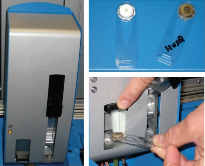
Figure 2. FPQ and XRF tower assembly
Combined Particle Quantifier (FPQ) and XRF Device
The modified pore blockage method has been called “Filtration Particle Quantification” or FPQ. The FPQ uses constant flow by driving a 3 ml oil sample using a syringe through a polycarbonate filter with approximately 30,000 4 µm diameter holes.
The resulting pressure drop across the filter is then measured with reference to atmospheric pressure and used to measure particles >4 µm up to ~ 1 million particles/ml. This is primarily achieved by using a modified filter design instead of a traditional pore blockage instrument.
This novel, patent-pending dual dynamic design enables a much greater particle count range (x50) beyond the point where particle swapping and saturation takes place (Figure 3).
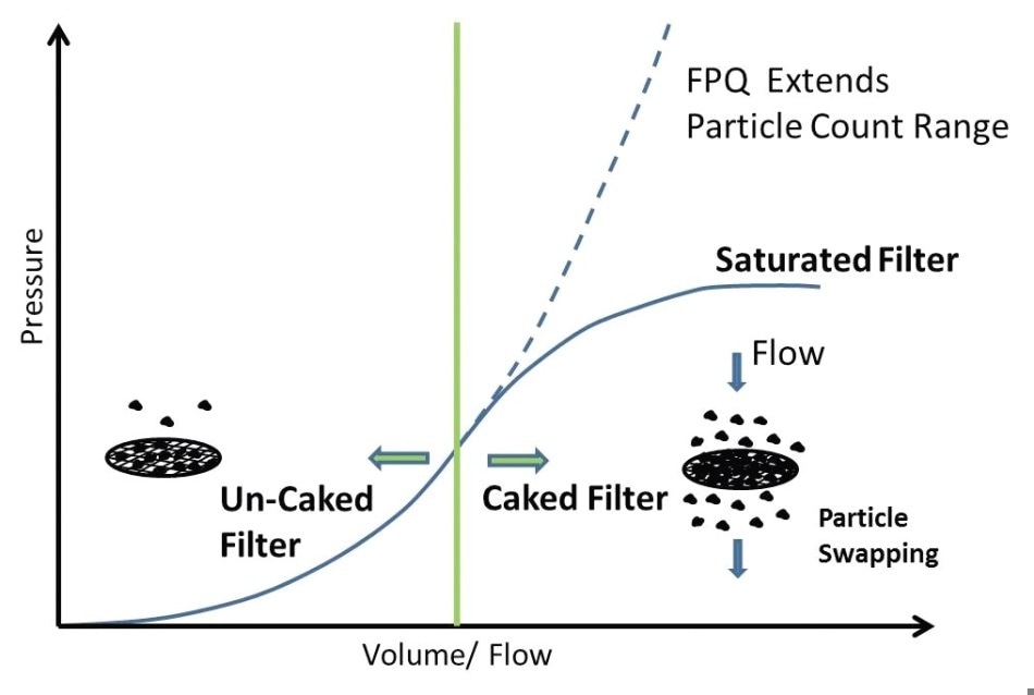
Figure 3. FPQ Filter vs Conventional Pore Blockage Filter
Once the analysis is complete, the filter passes from the FPQ to the XRF device. Due to the particle swapping phenomenon, the XRF and FPQ are closely linked in terms of calibration. A series of unique rules and calibrations are used by XRF and FPQ instruments to ensure accurate elemental quantification of particles up to 1 million particles /ml.
Combined with the patented filter, this method overcomes the problem associated with oil cup analysis, which are generally used by XRF devices. This filter design corrals the particles within a small area on the filter, so that the focused X-ray beam can concentrate its energy on those particles alone. The device employs 15 kev and 40 kev to quantify 13 elements with an average limit of detection of ~ 1 ppm.
FPQ / XRF Device Case Studies
The following case studies show how the XRF/FPQ instrument correlates to current analytical techniques for quantifying particles in different real world applications.
FPQ and X-Ray Correlation to Established Measurement Techniques
The FPQ and XRF technology was evaluated using the following data set from a series of marine diesel vessels. Samples were examined on XRF and the FPQ device, and were shown to correlate to LaserNet Fines® and acid digestion using the ICP spectrometer.
A model using an assumed particle mass and wear particle size aspect ratio was employed to further correlate the aggregate elemental concentration on the FPQ filter, using the LaserNet Fines® and XRF data. Figures 4 and 5 show how the XRF and FPQ correlate to the LaserNet Fines® direct imaging particle counter.
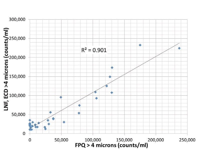
Figure 4. LaserNet Fines® vs. FPQ (counts/ml >4 µm)
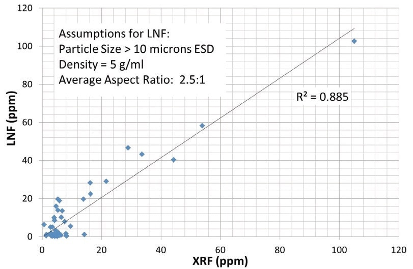
Figure 5. LaserNet Fines® vs. XRF – Total ppm
XRF vs. Acid Digestion
Spectroscopy and LaserNet Fines® direct imaging are proven techniques used to quantify elemental concentration and particle count, respectively. ICP and RDE spectrometers do not have the required sensitivity to detect large particles and they are employed as trending tools for fine particles based on a dissolved elemental calibration.
One established method to measure large particles is to “acid digest” the whole sample by dissolving the particles in a liquid, which can then be measured using a standard ICP calibration. However, acid digestion is impractical due to time, cost, effort, and corrosive chemicals.
A selection of marine samples, shown in Table 1, was examined on the ICP before and after acid digestion. This method is typically referred to as differential acid digestion.
Table 1. Differential Acid Digestion Sample Result (Sample E=10- 1151, SampeF=10-1149)
| |
Before Acid Digestion-ICP (ppm) |
After Acid Digestion-ICP (ppm) |
| Sample |
A |
B |
C |
D |
E |
F |
A |
B |
C |
D |
E |
F |
| Ag |
0 |
0 |
0 |
0 |
0 |
0 |
0 |
0 |
0 |
0 |
0 |
0 |
| Al |
0 |
0 |
0 |
10 |
10 |
21 |
0 |
0 |
0 |
0 |
13 |
28 |
| Cr |
6 |
0 |
0 |
0 |
6 |
7 |
6 |
0 |
0 |
0 |
6 |
8 |
| Cu |
0 |
0 |
0 |
0 |
11 |
11 |
0 |
0 |
0 |
0 |
10 |
10 |
| Fe |
10 |
7 |
0 |
0 |
33 |
67 |
11 |
10 |
0 |
0 |
35 |
86 |
| Mo |
0 |
0 |
0 |
0 |
0 |
0 |
0 |
0 |
0 |
0 |
0 |
0 |
| Ni |
0 |
0 |
0 |
0 |
0 |
0 |
0 |
0 |
0 |
0 |
0 |
0 |
| Pb |
0 |
0 |
0 |
0 |
0 |
0 |
0 |
0 |
0 |
0 |
0 |
0 |
| Sn |
0 |
0 |
0 |
0 |
0 |
0 |
0 |
0 |
0 |
0 |
0 |
0 |
| Ti |
0 |
0 |
0 |
0 |
0 |
0 |
0 |
0 |
0 |
0 |
0 |
0 |
| V |
0 |
0 |
0 |
0 |
0 |
0 |
0 |
0 |
0 |
0 |
0 |
0 |
| Total ppm |
16 |
7 |
0 |
10 |
60 |
106 |
17 |
10 |
0 |
0 |
64 |
132 |
Figure 6 shows how the differential ICP results (large particles) for samples E and F compared to the XRF data for the same samples. Note that the XRF data is not shown in Table 1. The portion of large particles correlates well (within 3 ppm) to the filtered XRF results (Figure 6).
Figure 7 shows the difference in ppm between the XRF and ICP readings for Al and Fe in Sample F. This is a predicted result based on the behavior of small and large particles in a closed loop lubricating system. Large particles get lost and filtered out much more easily compared to fine debris that is never lost and continues to increase in concentration.
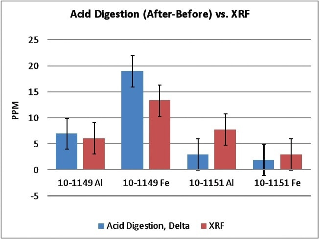
Figure 6. Differential ICP vs XRF (Sample E=10-1151, Sample F=10-1149)
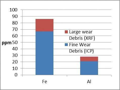
Figure 7. Typical ratio of large to small particles observed between XRF and ICP (Sample F)
PPM (mass) vs Particle Concentration (quantity) on the FPQ Filter
Based on the density of iron, it will take ~100 particles of the illustrated dimensions in 1 ml of oil to increase the elemental concentration by just 1 ppm. For lighter metals such as aluminum, it takes approximately three times the amount of particles. This shows why the differential elemental XRF and ICP readings are lower compared to the dissolved and fine particle readings using routine spectroscopy.
In this case, the Al and Fe wear particles are probably caused by piston/cylinder wear. This is a common failure mode in the application and demonstrates how the XRF can identify the root cause of problems.
Wear Progression to Failure
When a machine enters an abnormal wear mode there is always an increase in the production and size of severe large particles. They are identified as an increase from a known equilibrium level in the system. As the abnormal wear progresses, the size and rate of production of these particles also increases until the system eventually fails.
It must be noted that fine wear particles detected by ICP and RDE spectroscopy continue to rise in the lube system and are not affected by system loss mechanisms, including filtration. Care should be taken when changing the oil and subsequently interpreting XRF data versus fine and dissolved wear metal data.
Limits based on rate of change apply in this case. For larger particles quantified by XRF and FPQ, a static limit applies once the system reaches equilibrium, as shown in Figure 8.
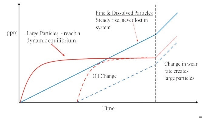
Figure 8. Behavior of large vs fine particles
The FPQ, unlike existing pore blockage and optical particle counter technologies, is capable of handling a range of applications with relatively high wear rates (up to 1.0 million p/ml). Table 2 lists the XRF and FPQ data for a variety of components that are generally found in transmissions, engines, final drives, front differential, and other heavy duty industrial vehicle equipment. The data shows pairs of components with corresponding low and high wear rates.
Table 2. Normal and abnormal FPQ & XRF data for various applications
| Sample |
Particles >4 µm (/ml) |
Application |
ITS Q5800 XRF (ppm) |
| laserNet Fines |
FPQ data |
Al |
Cu |
Fe |
Si |
| E1 High wear |
180209 |
141795 |
Engine |
2.0 |
0.0 |
0.8 |
1.4 |
| E2 Low Wear |
26802 |
44188 |
Ermine |
0.5 |
0.6 |
0.6 |
0.7 |
| T1 High Wear |
46618 |
50390 |
Transmission |
0.4 |
2.2 |
22 |
1.7 |
| T2 Low Wear |
5346 |
9664 |
Transmission |
0.0 |
0.0 |
0.2 |
0.3 |
| F1 High wear |
213674 |
226222 |
Final Drive |
4.3 |
0.0 |
8.4 |
7.0 |
| F2 Low Wear |
17185 |
26948 |
Final Drive |
0.1 |
0.0 |
2.0 |
0.5 |
| D1 HIgh Wear |
88193 |
62259 |
Front Diff |
1.2 |
0.0 |
4.2 |
1.9 |
| D2 Low Wear |
37613 |
34773 |
Front Diff |
0.9 |
0.7 |
2.9 |
1.2 |
| E3 High Water |
102532S |
31686 |
Engine |
0.5 |
0.0 |
1.0 |
0.4 |
The particle count on the FPQ correlates well with direct imaging particle counting (Figure 9), as predicted. Additionally, the elemental XRF readings are able to differentiate between more critical high wearing systems and low wearing systems. This data demonstrates that it is possible to make a recommendation on the root cause of the increased wear rates based on a material map of the lube system.
This data set also highlights a unique benefit provided by FPQ when studying emulsions and other types of samples that contain “phantom” particles in the overall particle count. Other liquids, including water pass through the polycarbonate filter pores without influencing the results.
A considerable amount of free water ingestion present in Sample E3 produced a highly elevated particle count reading on the LaserNet Fines®. In this sample, the real particle count was just ~ 31 k p/ml and the elemental level was low.
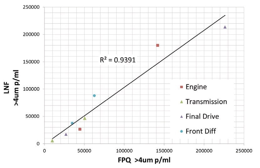
Figure 9. FPQ vs LaserNet Fines®, normal and abnormal wear in different applications
Conclusion
With its patent-pending dual dynamic filtration system, the FPQ handles a range of lubricant applications with varying levels of wear. The particle count using the FPQ filter correlates with current direct imaging particle counting. The following elemental concentration from the FPQ filter using XRF analysis correlates well with ICP differential acid digestion, indicating that the methodology is valid.
The combined elemental concentration and particle count not only detects the varying wear rates, but also isolates the possible root causes of problems in lube systems. Elemental concentration and particle count provide the true elemental break down of particles captured and measured on the filter. This method removes most of the issues that are associated with other methodologies such as particle size detection and also the impervious nature of many used oils found in heavy duty industrial applications.
References
1. Daniel P. Anderson and Richard D. Driver. “Equilibrium particle concentration in engine oil” Wear, Volume 56, Issue 2, October 1979, Pages 415-419
2. A.A., Bowen, E.R., and Westcott, V.C. “Characteristics of Particles Generated at the interface Between Sliding Steel Surfaces”Wear, Volume 34 (1975) Pages 261-273
3. Anderson, D.P., “Wear Particle Atlas (Revised)” prepared for the Naval Air Engineer¬ing Center, Lakehurst, NJ 08733, 28 June 1982, Report NAEC-92-163, Approved for Public Release; Distribution Unlimited – Pages 125-134

This information has been sourced, reviewed and adapted from materials provided by AMETEK Spectro Scientific.
For more information on this source, please visit AMETEK Spectro Scientific.