Superconducting Qubits for Quantum Computing

A quantum computer might be able to tackle computational problems that a classical computer can’t solve in practice [1, 2]. Such a device must fulfill certain criteria [3], such as the capability to initialize the state of its basic building blocks – the qubits – with high fidelity. A 10-fold speed-up in reset for a given fidelity is demonstrated, along with a 10-fold improvement for the final state preparation fidelity using an active reset method for superconducting qubits.

The method consists of a single-shot measurement of the qubit’s state followed by a conditional single qubit gate operation that rotates the qubit into the ground state if it was found in the excited state [4]. The method is compared with the simpler alternative for state initialization, passive waiting for qubit decay, and quantifying the speed and fidelity advantage of the active method. Speed is important for obtaining high experimental repetition rates.

The speed of the active method is generally limited by the achievable feedback latency. The speed of the passive method is restricted by the qubit lifetime making it impractical in view of the advances in fabrication leading to ever improving qubit lifetimes. The fidelity of the active method can exceed the limit set by the system temperature which applies to the passive method.

The chief issue in implementing active qubit reset is the need for low-latency signal processing and conditional signal generation. Zurich Instruments’ UHFLI allows feedback on the scale of a microsecond thanks to it incorporating a fast digital lock-in amplifier, an arbitrary waveform generator, and a cross-domain trigger engine joining the two. The UHFLI makes active qubit reset available without the cost of developing and maintaining a customized digital signal processing solution [4].

Setup and Sample

The sample utilized is shown in Figure 1 (a): it consists of niobium- and aluminum-based resonant circuits on a sapphire substrate [5]. The qubit shown in the inset is a nonlinear resonator formed of a small superconducting quantum interference device (SQUID) acting as a nonlinear inductor and an on-chip capacitor (orange in the image). The SQUID design makes the qubit frequency tunable over a frequency range from 4 to 7.5 GHz by applying a small magnetic field to the device.

A coplanar waveguide (green) guides external control signals to the qubit, which is attached to a coplanar-waveguide resonator (blue) [6] with a frequency of 4.78 GHz. This readout resonator is connected through an on-chip Purcell filter to a pair of coaxial cables that provide the interface for reading out the quantum state of the qubit. Figure 1 (b) depicts a schematic of the measurement setup in which the sample is placed in a dilution refrigerator, providing a well isolated low-temperature environment to protect the quantum properties of the sample.

Figure 1. (a) Optical micrograph of the sample showing the readout resonator (blue) and the qubit capacitor plates (orange). The resonator is coupled to input and output lines via a Purcell filter [7] (cyan). Insets show magnified views of the qubit and the coupler between resonator and Purcell filter. (b) Simplified diagram of the experimental setup based on the UHFLI instrument integrating a lock-in amplifier and an AWG. The superconducting qubit sample is cooled in a dilution refrigerator.

The control pulses are created by quadrature modulation of a microwave signal using two AWG channels. The pulses for qubit readout are generated by feeding one of the AWG marker channels to the gate input of a microwave frequency signal generator. After transmission through the readout resonator, the pulses are improved using a parametric amplifier followed by low-noise cryogenic and room-temperature amplifiers.

The signal is then down-converted in the analog domain to an intermediate frequency f_IF of 28.125 MHz. Employing one of the UHFLI lock-in amplifier channels, the signal is further down-converted in the digital domain. The resulting in-phase and quadrature component signals are then digitized utilizing the UHF-DIG Digitizer module of the UHF apparatus.

Qubit Rabi oscillation measurements were carried out [8] allowing the identification of the optimum set of parameters of the qubit π control pulse used to excite and reset the qubit. We used a first-order DRAG pulse shape as described in Ref. [9].

Active Qubit Reset

Single-Shot Qubit Measurement

Measuring of the original qubit state marks the beginning of the active qubit reset cycle. The qubit state is obtained by measuring the down-converted pulsed readout signal with the lock-in amplifier and likening the acquired quadrature voltage most sensitive to the qubit state change to a threshold value. The high-performance amplification chain based on the parametric amplifier enables a signal-to-noise ratio sufficiently large to discriminate the qubit states in a single shot without averaging over repeated experiments to be obtained.

The capability to achieve single-shot readout is a requirement for active qubit reset. Figure 2 displays the histogram of the measured signal quadratures over 40,000 repetitions of the same experiment. For the measurement in Figure 2 (a), no control pulse was used before the state measurement, and the qubit is therefore expected to be in thermal equilibrium close to the ground state (passive reset).

In Figure 2 (b), a π pulse was applied immediately before the state measurement, and here two local maxima matching the qubit ground and first excited states are identified, and a weaker maximum in the bottom half of the plot perhaps because of the population of the second excited state. The majority of the contrast for the state measurement is contained in the in-phase (I) signal component. We set the threshold for state discrimination to 1 mV (red vertical lines).

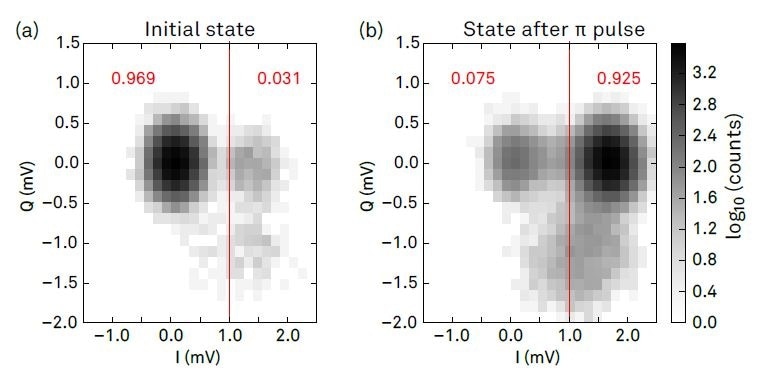
Figure 2. Histograms of integrated signal quadratures in repeated single-shot state measurement. (a) shows the histogram when measuring the qubit in its thermal equilibrium ground state after waiting a time much longer than the qubit lifetime before taking an individual measurement. (b) shows the histogram of measurements taken after having applied a π pulse to the qubit. The two maxima in the histogram in (a) and (b) are identified with the qubit’s ground and excited state, respectively. The red numbers are the relative fraction of counts in the areas delimited by red lines which represent the state discrimination threshold used for active qubit reset. The population of the ground state in (b) is mainly caused by relaxation during the readout.

Implementing Feedback with the UHF-AWG

The internal cross-domain trigger of the UHFLI was configured to perform the qubit state discrimination. The digital signal following this discrimination is used to define a sequence branching point in the UHF-AWG sequence program which determines whether the AWG will output a dual-channel π pulse, or no signal. The LabOne AWG Sequencer allows the formulation of the corresponding hardware instructions in an easily readable, high-level programming language called SeqC. The core part of that program is shown in Figure 3.

The first instruction in the program initiates the playback of the waveform w_read. This waveform has a digital marker that is employed as a gate signal to generate a readout microwave pulse. Following the playback, the sequencer is instructed to wait during wait_time until the cross-domain trigger engine has performed the state discrimination operation and the readout signal is obtainable. The binary result of the discrimination is then read by the sequencer and stored in the run-time variable qb_state.

The subsequent switch statement contains two branches, one of which is executed conditionally on the value of qb_state (0 or 1). One branch links to the dual-channel playback of the waveforms w_pi_1 and w_pi_2 (the qubit π pulse), the other to the playback of the zero-valued waveforms w_zero_1 and w_zero_2 of the same length. The waveforms in this part of the program are defined in the same program (not shown) using mathematical functions assessed by the compiler.

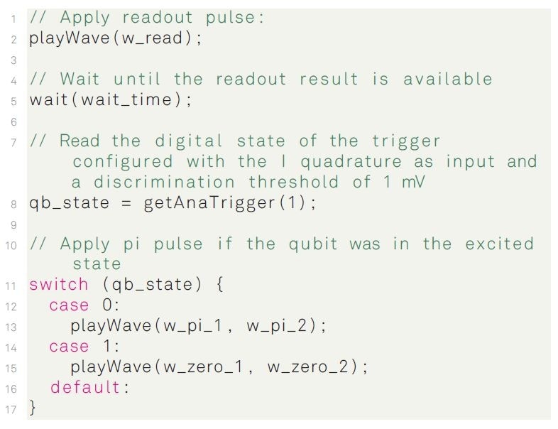
Figure 3. Core part of the sequence program in the SeqC language used to control the conditional feedback action.

Repeated Active Qubit Reset

The efficiency of the qubit reset can be increased by repeating the feedback cycle described above, allowing a sub-percent-level excited-state population to be achieved - better than what would be possible by using a single feedback cycle. Repetition of the cycle is done by looping over the code segment shown above.

The blue curve in Figure 4 illustrated the development of the qubit state during a qubit reset protocol consisting of 23 repetitions of a feedback cycle. The blue squares are the excited-state population averaged over 40,000 repetitions of the experiment. To compare the decay curve with the one observed without active reset, a control experiment was completed where the qubit state was read out repeatedly in the same way as with active reset enabled, but without a π pulse applied to the qubit. The decay curve without feedback, but with repeated measurements, is identical to a decay curve measured with a conventional T₁ measurement such as the one described in [8].

After the first feedback cycle or 1.48 µs, the qubit excited state population dropped to approximately 12%. Employing the passive method, achieving this level takes around 14 µs. After four to five replications, the initially fast decay gradually slows but the excited-state population continues to decrease. After 23 feedback repetitions, it has dropped to below 0.3%, while in the passive method the residual occupation converges to 3% after a long waiting time, also cf. the measurement in Figure 2 (a).

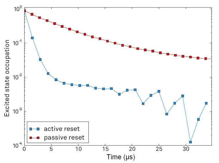
Figure 4. Time evolution of the averaged qubit excited-state occupation with active and passive qubit reset, respectively. Before the start of the protocol, the qubit is initialized by applying a π pulse. Every 1.48 microseconds, a state measurement is taken. After each measurement, a conditional π pulse is applied to initiate an active reset, or no pulse is applied for passive reset.

Feedback Latency

Feedback latency is critical in deducing the fidelity of the active qubit reset. A small latency lessens the main cause of error occurring during each feedback cycle, spontaneous qubit decay occurring between the readout and the π pulse. This mechanism accounts for about 19% error calculated from the qubit’s lifetime T₁ of 7.1 µs and the period 1.48 µs of one complete feedback cycle. Additionally, a small latency suggests more reset cycles can be accomplished in the same amount of time. In the following, measurements of the feedback latency in the configuration used for the experiment discussed above are discussed.

Figure 5 shows the setup used for these measurements. Compared to the setup in Figure 1, the wiring is altered so that the qubit control signals and the readout return signal are redirected to an oscilloscope. The UHFLI therefore doesn’t receive a readout signal, and the control signals generated by the UHF-AWG do not reach the qubit. As the signal processing latency in the UHFLI instrument is unaffected by these changes, however, the setup allows the observation of the same latency that would apply to the actual measurement, referenced to the plane of the UHFLI Signal Input and Output connectors.

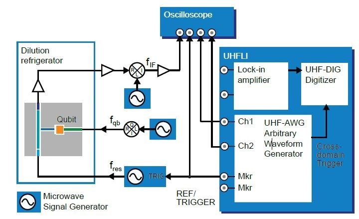
Figure 5. Setup used to measure the feedback latency of the active qubit reset. The qubit control signals and the qubit readout signals are routed with cables of equal length from the UHFLI to an oscilloscope. The gate signal generated by the UHF-AWG marker channel 1 is connected to the oscilloscope via a T-piece for triggering. The UHFAWG Sequencer executes the same program as in the experiment, which makes the timing in this measurement equal to the timing in the actual experiment.

Figure 6 shows the qubit readout and control signals measured in the configurations. The readout signal (top) at the intermediate frequency is averaged over multiple scope acquisitions in order to make its timing clearly visible despite the noise. From the beginning of the readout signal burst to the start of the qubit control pulses generated by the AWG, a latency of 1.12 µs was measured. Part of this time is the signal integration time of 0.37 µs that allowed a sufficiently high SNR for the single-shot readout to be obtained. The remainder, about 0.75 µs, is from other signal processing such as A/D and D/A conversion or demodulation and signifies the minimum latency achievable with the UHF instrument.

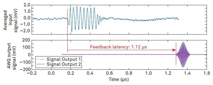
Figure 6. Measurement of the feedback latency of the UHF instrument referenced to its front panel connectors. The dual-channel AWG signal starts 1.12 μs after the start of the readout pulse. The input signal has been averaged in order to identify the start of the readout pulse using an oscilloscope.

Conclusion

The measurements shown quantify the benefits of the active qubit reset method and determine the ease of its implementation with the UHFLI Lock-in Amplifier and the UHF-AWG Arbitrary Waveform Generator. A ten-fold speed-up in reset for a given fidelity and a ten-fold improvement for the final state preparation fidelity was achieved compared to the passive reset method.

These results build on powerful, low-latency digital signal processing tools available on the Zurich Instruments UHF instrument. Flexible extension to multi-qubit measurement and control systems is facilitated by the possibility to achieve demodulation at multiple frequencies with the UHF-MF option. Multiple AWG sequence branches also allow for more complex feedback protocols, e.g. taking into account detection of higher excited states.

Acknowledgments

Zurich Instruments would like to thank Prof. Wallraff and the members of his Quantum Device Lab at ETH Zurich, Switzerland, in which these measurements were carried out. Special thanks go to Michele Collodo. We thank Theodore Walter for providing the qubit sample and Yves Salathé, Simone Gasparinetti, and Philipp Kurpiers for support with the measurements and for discussions. This work was supported by the Swiss Federal Department of Economic Affairs, Education and Research through the Commision for Technology and Innovation (CTI).

References

1. R. P. Feynman. Simulating physics with computers. Int.J.ofTheor.Phys.,21:467,1982.
2. T.D. Ladd, F. Jelezko, R. Laflamme, Y. Nakamura, C. Monroe, and J.L. O’Brien. Quantum computers. Nature,464:45,2010.
3. David P. DiVincenzo. The physical implementation of quantum computation. arXiv:quantph/0002077,2000.
4. D. Ristè, C. C. Bultink, K. W. Lehnert, and L. DiCarlo. Feedback control of a solid-state qubit using high-fidelity projective measurement. Phys. Rev.Lett.,109:240502,2012.
5. T. Walter, P. Kurpiers, S. Gasparinetti, P. Magnard, A. Potocnik, Y. Salathé, M. Pechal, M. Mondal, M. Oppliger, C. Eichler, and A. Wallraff. Rapid high-fidelity single-shot dispersive readout of superconducting qubits. Phys. Rev. Applied, 7:054020, May 2017.
6. A. Wallraff, D. I. Schuster, A. Blais, L. Frunzio, R.S. Huang, J. Majer, S. Kumar, S.M. Girvin, and R.J. Schoelkopf. Strong coupling of a single photon to a superconducting qubit using circuit quantum electrodynamics. Nature,431:1627,2004.
7. M.D. Reed, B.R. Johnson, A.A. Houck, L. DiCarlo, J. M. Chow, D. I. Schuster, L. Frunzio, and R. J. Schoelkopf. Fast reset and suppressing spontaneous emission of a superconducting qubit. Applied Physics Letters,96:203110,2010.
8. Zurich Instruments AG. Superconducting Qubit Characterization,2016. Application Note.
9. F. Motzoi, J.M. Gambetta, P. Rebentrost, and F.K. Wilhelm. Simple pulses for elimination of leakage in weakly nonlinear qubits. Phys. Rev. Lett., 103:110501,2009.

This information has been sourced, reviewed and adapted from materials provided by Zurich Instruments.

For more information on this source, please visit Zurich Instruments.