Rheometry is the method used to analyze the rheological behavior of a material; with rheology defined as the study of matter when it flows or is deformed. As a result rheology describes forces and deformations over time.
The term rheology, as with most scientific fields, has its roots in Ancient Greek with the stem rheo meaning ‘flow’ in English. As the field has advanced it is no longer just concerned with the flow of liquids but also the deformation of solids and the complex behavior of viscoelastic materials that have the properties of both liquids and solids depending on the forces/deformations applied to them.
Several different rheometric measurements can be carried out using a rheometer to measure the rheological behavior of a sample that this article will cover separately. The article will firstly cover the testing of simple and complex fluids, followed by deformation and viscoelastic testing.
Viscosity
Flow can be either shear, where fluid components shear past one another, or extensional, where fluid components either flow towards or away from each other. Most flow occurs via a shear mechanism, and this can be easily measured using a rotational rheometer.
Shear Flow
Shear flow can be described as several layers of fluid sliding over each other, with each upper layer moving faster than the layer below it. The bottom layer of the fluid is considered to be stationary and the top layer has the highest velocity. Sheer flow occurs due to the application of a shear force on the fluid.
The external shear force is described mathematically (Figure 1) as the shear stress (σ), which is the force (F) applied over a unit area (A). As the top layer responds the most to this force, and the bottom layer doesn’t respond at all, a displacement gradient is formed through the sample (x/h), which is called the sheer strain (γ).
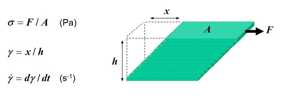
Figure 1 – Quantification of shear rate and shear stress for layers of fluid sliding over one another.
For classical solids, i.e. those that behave as a single block of material, when stress is applied the strain in infinite meaning that flow is impossible. For fluids, where components can flow past one another, the sheer strain increases over the time that the strain is applied. This increase results in a velocity gradient, which is called the sheer rate (v) and is given as a differential of strain with respect to time (dγ/dt).
The application of a shear stress to a fluid involves the transfer of momentum; with the shear stress being equal to the rate of momentum transfer (momentum flux) to the fluid’s upper layer. This momentum is transferred downwards through the fluid layers with a reduction in kinetic energy, and therefore layer velocity, between layers due to collisional energetic losses.
The coefficient of proportionality between the shear rate and the shear stress is described by the shear viscosity, aka the dynamic viscosity, (η). The shear viscosity describes the internal friction of the fluid between its layers and a greater sheer viscosity results in damping, i.e. losses of kinetic energy in the system.
Newtonian fluids are fluids that have a linear relationship between the shear rate and the shear stress meaning that the viscosity is invariable. Everyday Newtonian fluids include examples such as water, dilute colloidal dispersions, and simple hydrocarbons.
Non-Newtonian fluids are fluids that have a non-linear relationship, i.e. the viscosity varies as function of the applied shear stress or shear rate.
Viscosity is also temperature and pressure dependent. Viscosity tends to increase as the pressure increases (as layers are pushed together) and as the temperature increases. Temperature has the greater impact out of the two with very viscous fluids such as bitumen or asphalt showing more temperature dependency than less viscous fluids, such as simple hydrocarbons.
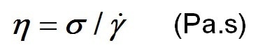
Measurement of the shear viscosity with a single head (stress controlled) rotational viscometer takes place as follows. The sample is loaded between two parallel plates with an exact gap (h) between them (Figure 2). Single head rheometers can be set up for either controlled rate measurement (where a rotational speed is applied and the torque required to maintain the speed is applied) or controlled stress measurement (where a torque is applied and the rotational speed is measured).
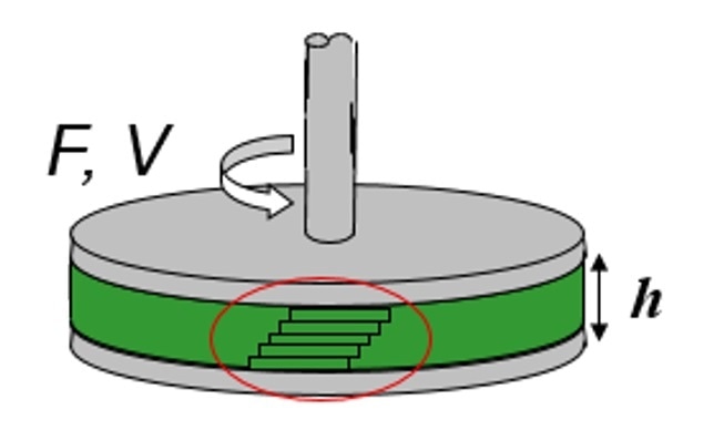
Figure 2 – Illustration showing a sample loaded between parallel plates and shear profile generated across the gap.
For controlled stress measurements the motor drives a torque which is transferred to a force (F) which is applied to the liquid over the plates area (A) to give a shear stress (F/A). The application of the shear stress results in the liquid flowing at a shear rate, which is viscosity dependent. As the gap between the plates (h) is known the shear rate can be calculated (V/h) using the sum of the angular viscosity (ω) of the upper plate, which is measured by sensors and the plate radius (r), because V = r ω.
Other types of measuring systems are frequently used for the measurement of viscosity, such as cone-plate and concentric cylinder systems. Cone-plate systems are popular because they provide a consistent shear rate over a sample.
The sample type and its viscosity range often determine the measurement system used. For example, low viscosity and volatile fluids are ideally measured in a double gap concentric cylinder, and large particle suspensions should not be measured in a cone plate system.
Shear Thinning
The most commonly seen type of non-Newtonian behavior is shear thinning, aka pseudoplastic flow. During shear thinning the viscosity of the fluid reduces as the shear increases. At a low enough shear rate fluids, which exhibit shear thinning will have a constant viscosity, η0 – the zero shear viscosity. At a critical point a significant drop in viscosity occurs which marks the beginning of the region of shear thinning behavior.
Why Does Shear Thinning Occur?
Shear thinning occurs because of rearrangements in the fluid microstructure in the plane of the applied shear. It is frequently seen in dispersions such as suspensions and emulsions, including melts and solutions of polymers. Figure 3 shows different types of shear-induced orientations that are present in materials that exhibit shear thinning.
Figure 3 - Illustration showing how different micro-structures might respond to the application of shear.
Model Fitting
The different features of flow curves, which are illustrated in Figure 3, can be modeled using relatively simple equations. This approach allows the shape and curvature of flow curves to be compared to one another using only a small number of parameters.
This allows the prediction of flow behavior at shear rates for which data is not available, though care must be taken when drawing conclusions from data that is extrapolated.
Three of the most popular methods of fitting flow curves are the Power law, Cross and Sisko models. Which model is most appropriate depends on the region of the curve to be modeled and the data range available (Figure 4).
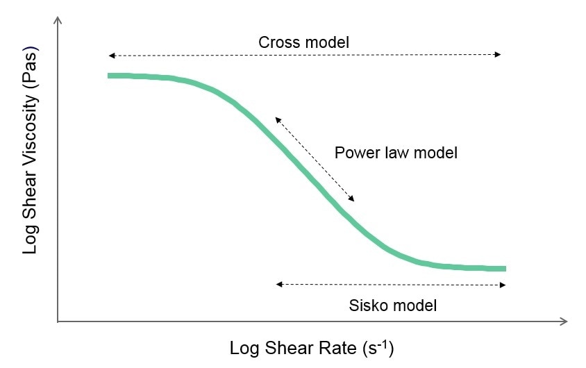
Figure 4 – Illustration of a flow curve and the relevant models for describing its shape.
There are also other models available, for example the Ellis model and Careau-Yasuda model, and also models that include yield stress such as the Herschel-Bulkley, Casson, and Bingham models.
Shear Thickening
The majority of polymer-based materials and suspensions display only shear thinning, though some can also show behavior where viscosity increases as the shear stress or rate increases – this behavior is called shear thickening.
Shear thickening is also known as dilatancy. Technically dilatancy refers to be a specific mechanism by which shear thickening occurs (which has an associated increase in volume) though the two terms tend to be used interchangeably.
Thixotropy
In the majority of the liquids shear-thinning behavior is completely reversible, with the liquid returning to its ‘normal’ viscosity once the force is removed. If this relaxation is time-dependent then the fluid is called thixotropic.
Thixotropy is the result of the time-dependent rearrangement of microstructures within the shear-thinning fluid after a significant change in the shear applied (Figure 5). Shear thinning materials can be thixotropic whereas thixotropic materials are always shear thinning.
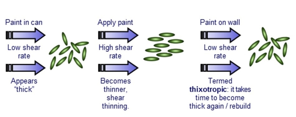
Figure 5 – Illustration showing micro-structural changes occurring in a dispersion of irregularly shaped particles in response to variable shear.
An example of a thixotropic material is paint. Paint when left sitting in the can is very thick and viscous, as this prevents de-emulsification, but following stirring should exhibit lower viscosity (i.e. shear-thinning) to make it thinner and easier to apply. When stirring is stopped there is a time lag before it becomes thick and viscous again, over which its structure rebuilds – this is thixotropic behavior.
Yield Stress
A large number of shear-thinning fluids exhibit the properties of both classical fluids and solids. When at rest these fluids form interparticle/intermolecular networks via the tangling of their polymers or intermolecular associations. This networked structure means the particles exhibit solid behavior such as elasticity. The extent of this behavior is determined by the forces holding the network together (the binding force) and therefore the yield stress.
Viscoelasticity
Viscoelastic behavior, as indicated by the name, is where materials exhibit behavior somewhere between a classical solid (elasticity) and a classical liquid (viscosity).
Visoelastic materials can be tested using one of several rheometric methods such as stress relaxation, oscillatory testing or creep testing.
Elastic Behavior
Viscous Behavior
In the same way that a spring can be used as a model to describe the behavior of a linear solid which follows Hooke’s law, viscous materials can be considered to behave in a similar fashion to a dashpot which follows Newton’s law. Dashpots are mechanical systems which possess a plunger which can be pushed into a viscous Newtonian fluid.
If a force/stress is applied to the dashpot then it begins to deform, and this deformation occurs over a constant rate, the strain rate, until the force is no longer applied (Figure 6). The energy needed to provide displacement/deformation is lost within the fluid (mostly as heat) and the applied strain is permanent.
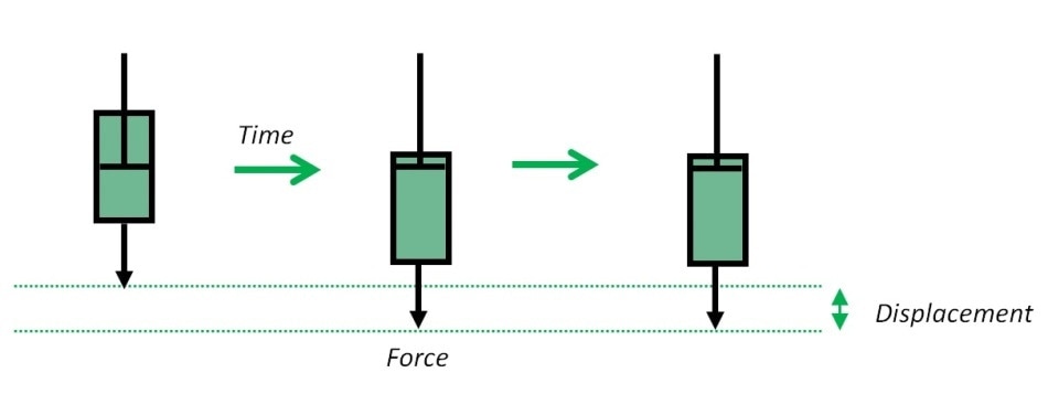
Figure 6 – Response of an ideal liquid (dashpot) to the application and subsequent removal of a strain inducing force.
Viscoelastic Behavior
A large majority of materials exhibit rheological behavior, which is in between liquid and solid behavior, and for this reason they are called viscoelastic materials. In order to describe the behavior of these materials through a model a combination of springs (to describe solid behavior) and dashpots (to describe liquid behavior) can be used.
The most basic form of this spring-dashpot model is the Maxwell model which involves the connection of a spring and a dashpot in series. The Kelvin-Voigt model can also be used to describe viscoelastic solids, which also uses springs and dashpots but connects them in parallel instead (Figure 7, mentioned at end too).
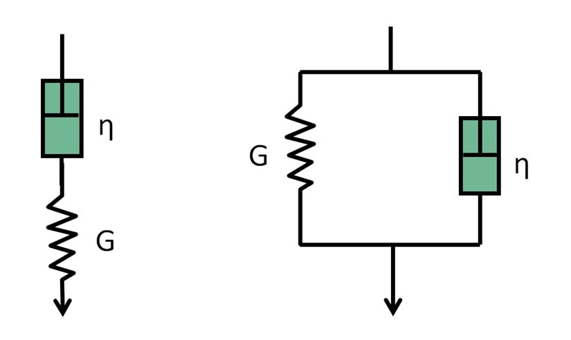
Figure 7 – (left) Maxwell model representative of a simple viscoelastic liquid; (right) Kelvin-Voigt model representative of a simple viscoelastic solid.
Creep Testing
Creep tests involve the application of a constant force to an elastic material, followed by the measurement of its strain response. Creep tests are most often used on materials, which creep, i.e. flow very slowly, over an extremely long timescale. Examples of these materials include metals and glass. That said, creep tests can be applied to many different types of viscoelastic materials in order to find out more about their behaviors and internal structures.
Creep testing involves the application of a constant shear stress over a set time period with measurement of the shear strain created as a result. Creep testing must take place in the materials linear viscoelastic region, i.e. where the material’s microstructure is present.
Small Amplitude Oscillatory Testing
The most frequently used method, which uses a rotational rheometer, for the measurement of viscoelastic behavior is small amplitude oscillatory shear (SAOS) testing. SAOS testing involves oscillating a sample around its resting state (called the equilibrium position) in a continuous cycle. As oscillatory motion is mathematically very similar to circular motion a full cycle is equal to a revolution through 2π radian, i.e. 360°.
The amplitude of the oscillation is equal to the maximum force (stress or strain) applied to the sample whereas the number of oscillations per second is given as the angular frequency.
Linear Viscoelastic Region (LVER)
When taking measurements of viscoelastic behavior such as the ones covered above it is highly important that the measurements are taken when the sample is displaying behavior in its viscoelastic region, i.e. where the strain and stress are proportional to one another.
When a material is in its LVER the application of stress does not result in breakdowns of material microstructure (called yielding), which means that the microstructural properties of the material can be determined.
If the stress is sufficiently high to cause the material to yield then non-linear relationships between the parameters will begin to appear which makes it difficult, and inaccurate, to correlate the measurements to the materials microstructure.
Determination of where the LVER of a material lies can be carried out via stress or strain sweep testing and determining the point at which the material yields (Figure 8). This is the point at which G’ exhibits stress or strain dependency.
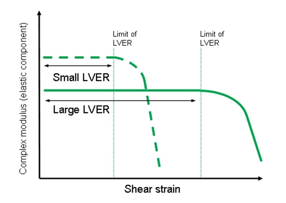
Figure 8 – Illustration showing the LVER for different materials as a function of applied strain.
Oscillatory Frequency Sweep
Viscoelastic materials exhibit different behavior depending on the time they have been left to rest, and for this reason G’ and G” cannot be considered as material constants.
In creep testing the extent of time dependence can be determined by measuring the creep compliance with respect to the time period stress was applied for. If an oscillatory method is used the extent of time dependence can be determined by altering the frequency of the applied strain or stress. Using this method low frequencies correspond to longer timescales, and high frequencies correspond to shorter timescales, because ω ≈ 1/t.
Carrying out a frequency sweep on a visoelastic material (which exhibits behavior following the Maxwell model) provides a plot such as that in Figure 9. As G’ and G’’ can vary for a Maxwell model.
A frequency sweep performed on a viscoelastic liquid (representative of Maxwell type behavior) yields a plot of the type shown in Figure 9.
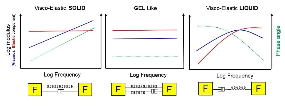
Figure 9 – Typical frequency response for a viscoelastic solid, viscoelastic liquid and a gel in oscillatory testing.
The Viscoelastic Spectrum
The viscoelastic behavior of real materials can be described using a combination of the Maxwell and Voigt models, such as the Burgers model (Figure 7). The Maxwell model describes behavior at low frequencies, and the Voigt model at high frequencies.
For an entangled polymer system the expected viscoelastic spectrum over a frequency range is illustrated in Figure 10. Often only a section of this whole spectrum can be observed for a specific material when using conventional rheometric methods, which are dependent on the instrument sensitivity and the time take for the material to relax.
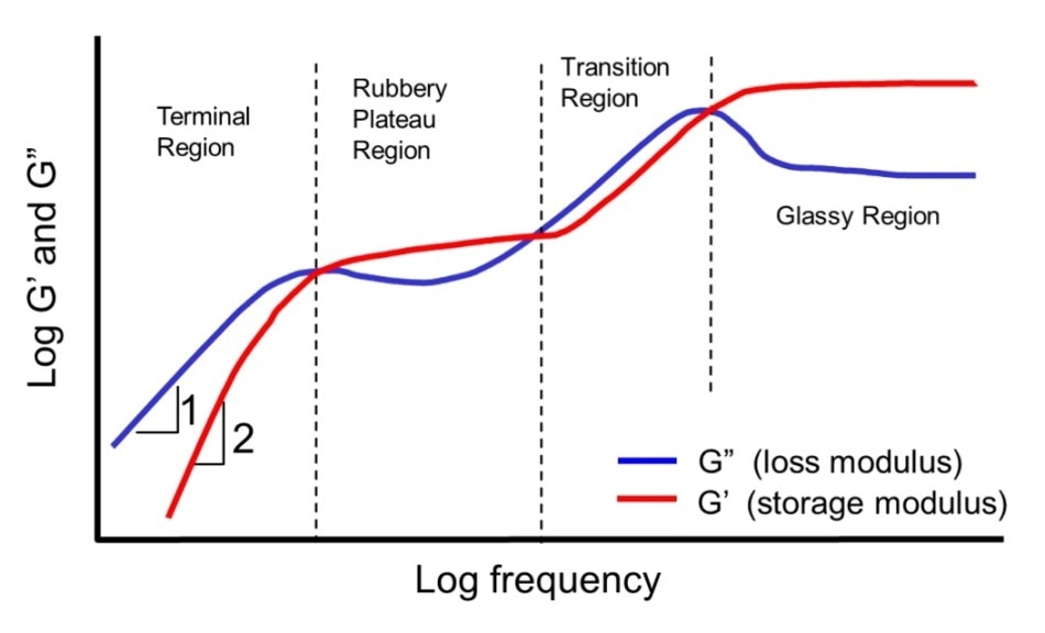
Figure 10 – A typical viscoelastic spectrum for an entangled polymer system.
References
- Barnes HA; Handbook of Elementary Rheology, Institute of Non-Newtonian Fluid Mechanics, University of Wales (2000)
- Shaw MT, Macknight WJ; Introduction to Polymer Viscoelasticity, Wiley (2005)
- Larson RG; The Structure and Rheology of Complex Fluids, Oxford University Press, New York (1999)
- Rohn CL; Analytical Polymer Rheology – Structure-Processing-Property Relationships Hanser-Gardner Publishers (1995)
- Malvern Panalytical White Paper- Understanding Yield Stress Measurements – https://www.malvernpanalytical.com/en
- Larsson M, Duffy J; An Overview of Measurement Techniques for Determination of Yield Stress, Annual Transactions of the Nordic Rheology Society Vol 21 (2013)
- Malvern Panalytical Application Note - Suspension stability; Why particle size, zeta potential andrheology are important
- Malvern Panalytical White Paper - An Introduction to DLS Microrheology.
- Duffy JJ, Rega CA, Jack R, Amin S; An algebraic approach for determining viscoelastic moduli from creep compliance through application of the Generalised Stokes-Einstein relation and Burgers model, Appl. Rheol. 26:1 (2016)

This information has been sourced, reviewed and adapted from materials provided by Malvern Panalytical.
For more information on this source, please visit Malvern Panalytical