How White Light Interferometry Can Measure Surface Roughness

Almost a century ago the concept of measuring surface roughness started as a way to stop disputes and uncertainty between buyers and manufacturers.

Today, it is a common identifier that is utilized across industry for confirming adherence to both internal and regulatory specifications, validating manufacturing processes, and guaranteeing performance and quality of end products.

Subjective judgments of quality that are based on finger touch feel or naked eye observation of surfaces have slowly been replaced by well-defined formulas and unbiased metrics. Mean roughness (Ra) was the first parameter developed for these attempts, which is still a primary reference parameter used today for a number of reasons.

First, mean roughness is easy to calculate, even using an analog method, which was crucial in early implementation across a variety of industries and also makes it a convenient and fast technique for current characterization.

Secondly, the Ra parameter is a robust calculation that averages outlier data and supplies constant results irrespective of the roughness pattern. This is extremely crucial, not only to assist with a large scope of industrial manufacturing processes but also to supply a solid baseline for process improvement.

The use of Ra as a key parameter to qualify surface roughness relies on defined standard samples (standards) of the desired profile measurement. These are fairly simple to manufacture for a single line profile and are frequently utilized to check if a roughness measurement system is calibrated properly.

This ensures that the Ra value provided for a specific surface is linked back to a well established reference value. These standards also help to achieve a common reference across multi-industrial sites and supply tool-to-tool correlation in multi-metrology systems.

While originally, these standards were designed for the single-line measurements of stylus-based profilers, they can also verify that both non-contact and contact areal-based profilers gather the correct results.

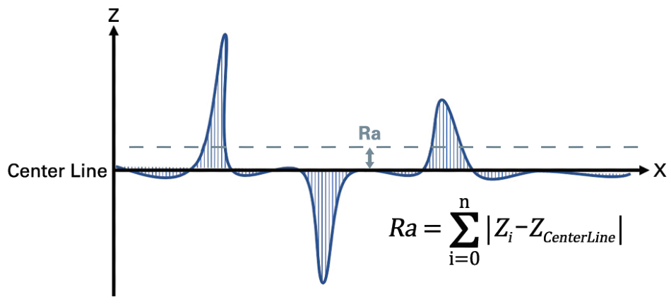
Figure 1. Illustration of mean roughness calculation. Image Credit: Bruker Nano Surfaces

This article outlines the utilization of mean roughness measurements with white light interferometry (WLI) optical profilers. Spatial filters are discussed, in addition to some of the normative standards requirements from ASME B46.1-2009,¹ ISO 13565-1² and JIS B 0671-1.³

The key technical reasons for WLI choice are covered, in addition to the benefits and areas of applicability of the full areal measurement standard from ISO 25178-2.⁴

Roughness and Spatial Filtering

In manufacturing, products are defined via key dimensions summarized into technical drawings. Roughness is one specific critical parameter that determines how much a surface measurement deviates from a specified form or shape, with height variation within the millimeter lateral range.

Part of another parameter, waviness, is larger fluctuation in topography. The surface of a product is the aggregate of shape, form, waviness, and roughness, all defined to a desired volume. In this way, roughness can only be calculated after the proper selection of spatial components, excluding form, shape, and waviness.

Roughness measurements always include step, where shape is removed, either via post-processing (e.g., high-order polynomial fitting and/or spatial filtering), or directly via a physical skid (as with some stylus profilers).

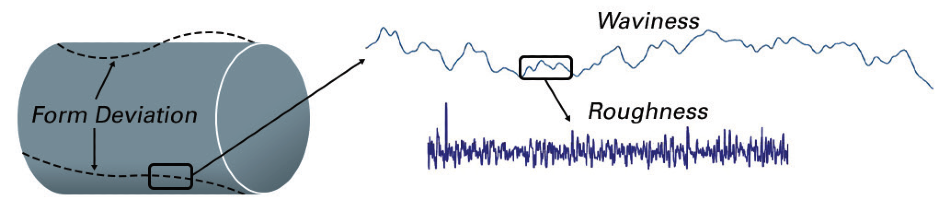
Figure 2. Determining roughness for a cylindrical part. Image Credit: Bruker Nano Surfaces

In the first instance, long-range topography fluctuations or equivalent low spatial frequencies are leveraged out using a high-pass filter, which only permits fast topological variation to pass through.

Vice-versa, short rapid variation on a profile usually signals the presence of noise, which should not be considered for a roughness measurement. In these instances, the high spatial frequencies are excluded via a low-pass filter.

So, raw measurement profiles go through band-pass filters for higher and lower spatial limits. Those boundaries are defined as λc and λs cut-off parameters in ISO 4287 and ASME 46.1 norms.

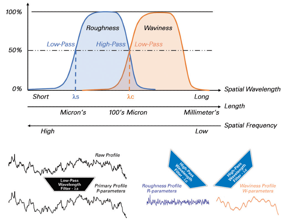
Figure 3. Spatial filter definition with associated derived parameters and resulting profiles. Image Credit: Bruker Nano Surfaces

While filtering is a vital part of measuring roughness, it should be considered that filters may also distort measured topography. For instance, the traditional employment of RC filters was well-known for triggering edge effects which needed exclusion bands to be used at the start and end of profiles in order to remove spurious data.

RC filters are also susceptible to distort topography around sudden height variations, like peaks or pits. So, this filter has been mainly replaced in current usage by more reliable filters, like spline-phase-compensated and Gaussian filters.

Recently, the growing utilization of areal roughness has sparked the requirement for even further advanced filters, like Robust Gaussian Filters,⁵ which are part of the ISO 25178 norm. These filters supply a unique benefit for avoiding edge effects.

This enables a roughness calculation by the effective removal of waviness over the entire measurement field while capturing fine variations in topography accurately.

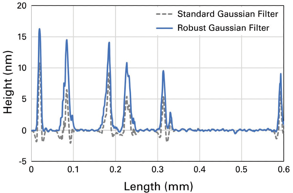
Figure 4. Plot showing the advantage of a spatial filter. Image Credit: Bruker Nano Surfaces

Profile Versus Areal Measurements

Stylus-based profiles have captured mean roughness and assessed the quality of parts successfully for nearly a century. Common turning, milling, and other CNC machining processes all leave well-defined direction where roughness happens.

In these instances, dragging the stylus perpendicularly to the main machining traces allows precise and reliable measurement of a surface's texture. This type of measurement is now known as a 1D type, where height (Z) is expressed versus scanning length (X).

However, over the last two decades, a higher level of complexity for surface metrology has been driven by the need for higher manufacturing efficiency and both cost and energy savings. Surfaces are now engineered to serve specific purposes, making the roughness parameter an even more crucial parameter for most precision-engineered parts.

In order to enhance performance, or to improve lifetime or wettability, surfaces are textured in various directions (e.g., with a lower coefficient of friction). Each of these processes are difficult to assess with a single-line profile, making multi-site measurements and a better statistical technique necessary.

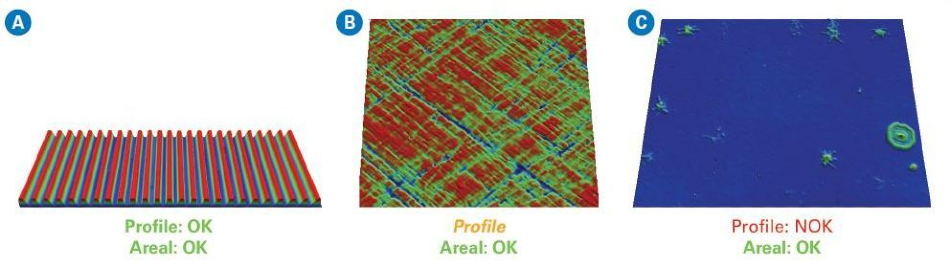
Figure 5. Three types of surfaces showing different applicability for profiler or areal topography measurements: (A) profile roughness standard; (B) cross-hatch texture on bore cylinder; and (C) defects on an optical window. Image Credit: Bruker Nano Surfaces

Full areal roughness metrology, known as 2D measurements, have become the most common means of characterizing surface roughness, due to these growing limitations in pure 1D roughness measurements.

These measurements plot vertical height versus X and Y directions. The first methods available were also based on stylus profiler capabilities, combining numerous adjacent lines into one area.

For this technique, the main drawbacks were the long measurement times, typically an hour or more to acquire high lateral resolution in both directions, plus the inherent fluctuation between each line because of mechanical drift.

Numerous groups were successful in using optical microscopes to measure topography in the 90s, based on interferometry techniques.⁶ This allowed quick (seconds to minutes) non-contact roughness measurements.

Areal roughness measurement methods have grown since then, to include confocal,⁷ focus variation,⁸ and digital microscope techniques. These methods all capture the full field of view and work out a dedicated height position for each pixel of an image. They are now known as 2D (area).

It should be considered that there are also 3D methods that measure full volume, including re-entrant and porous surface (e.g., confocal X-ray tomography). Yet, these approaches excel at different parameters than surface roughness.

It becomes much more simple to capture surface texture in all directions with a 2D or areal measurement, in addition to identifying any random defect along a surface.

It also gathers a larger field, which makes measurements more robust through the higher amount of statistical data available, in addition to more representative of overall surface texture.

1D and 2D measurement methods co-exist in modern industry. Mean roughness can easily be captured through a few profiles for standard manufacturing processes that leave a single texture orientation.

Both stylus profiling and areal measurements are valid if a texture has two or more orientations; with stylus profiling needing multiple lines, more time, and more statistical analysis to present the surface accurately.

Lastly, optical areal measurement becomes mandatory to properly evaluate the surface in the case of random and/or a complex engineered texture.

White Light Interferometry Profiler

Non-contact areal profilers are widely used to measure roughness in both R&D and production environments, due to the heightened complexity of much manufacturing today. Various design variations exist, but they usually share a design with a dedicated rigid structure that acts as a platform for high-end objectives and digital cameras.

They also share the fact that vertical and lateral resolutions are objective dependent, which has resulted in the common employment of highly resolutive objectives with short working distances for optimum vertical resolution.

The WLI-based profilers are a major exception to this trend, where vertical resolution not only becomes independent from the objective but it also reaches uniquely sub-nanometer levels. A WLI profiler uses interferometric objectives that show the sample surface via a moiré pattern only when proper focus is attained.

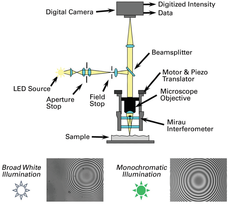
Figure 6. WLI optical implementation with display of different Moiré pattern versus illumination. Image Credit: Bruker Nano Surfaces

The focal plane can be easily worked out through finding the maxima within a couple of nanometers, as the depth of field for the moiré presence is not over ±0.5 µm because of the limited coherence length of white light illumination.

This sharp determination of focal plane is independent from the objective and relies completely on moiré, which even with low-magnification objectives (e.g., 1x, 2.5x, or 5x), guarantees nanometer precision. There are multiple advantages of this method:

• Ease of utilization is heightened with the extra safety margin between objective and surface, plus the ability to target challenging locations
• A mirror can be inserted along the focusing beam to deflect the optical path to measure vertical walls with better precision
• Since all objectives have the same vertical precision, budget allocation and metrology assessment become easier
• Long-working-distance objectives can be used without compromising vertical resolution to access specific or recessed locations on a complex part
• Stitching can be employed to combine high lateral resolution across even wider areas
• If low lateral resolution is required, a single acquisition at low magnification covers a wide range (100 mm²), permitting high throughput flatness control, or making fast detection of defects possible

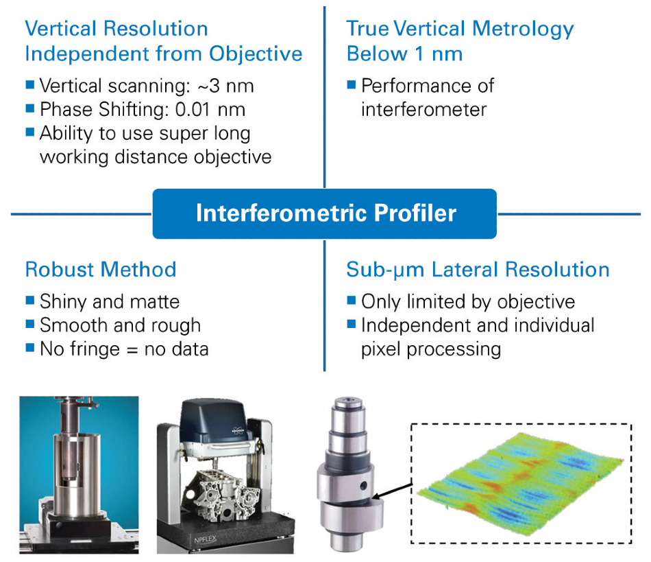
Figure 7. Attributes of WLI metrology. Image Credit: Bruker Nano Surfaces

Not only does a WLI-based profiler comply, and is listed as an appropriate method for areal norm ISO 25178-204:2013, due its unique vertical resolution, it is also being utilized by major reference metrology laboratories (PTB, NIST, NPL, et al.) to calibrate for artifacts.

Some advanced WLI profiler designs use a direct reference to a stabilized HeNe laser⁹ for automatic and self-calibration purposes based on this work.

Roughness Calculations

In addition to filtering, the ASME B46.1, ISO 11562-1997, and JIS B 0632:2001 standards clearly define measurement conditions for surface profiles. The raw profile is corrected for shape before the roughness calculation.

Next it goes through a low-pass filter established by cut-off λs to acquire the primary profile, P. After further high-pass filters defined by cutoff λc, to remove waviness roughness parameters are calculated.

Using this roughness filtered profile, all R parameters are determined. The filters are defined by mathematical function; most often Gaussian or splinephase corrected. For periodic profiles (e.g., turning, milling, etc.), both cut-off parameters are set to expected mean roughness for random surfaces or with spacing between peaks (see Table 1).

Table 1. Measurement and spatial filter conditions versus expected profile roughness. Source: Bruker Nano Surfaces

Periodic Profile	Non Periodic Profiles		Cut-off		Cut-off Ratio	Evaluation Length	Stylus
Spacing Distance RSm (mm)	Rz (µm)	Ra (µm)	λc (mm)	λs (µm)	λc/λs	Lm (mm)	Radius (µm)
>0.013 to 0.04	to 0.1	to 0.02	0.08	2.5	30	0.4	2
>0.04 to 0.13	>0.1 to 0.5	>0.02 to 0.1	0.25	2.5	100	1.25	2
>0.13 to 0.4	>0.5 to 10	>0.1 to 2	0.8	2.5	300	4	2 (5@Rz>3 µm
>0.4 to 1.3	>10-50	>2 to 10	2.5	8	300	12.5	5 or 2
>1.3 to 4.0	>50	>50	8	25	300	40	10, 5 or 2

 

Using the cut-off values, standards derive the exact measurement travel (Lt), which includes evaluation length (Lm) extended by pre- and post-lengths. In the instance of a Gaussian filter, pre- and post-lengths correspond to λc/2 length to decrease the influence of potential mechanical backlash at the beginning and end of a scan, in addition to filter edge effects.

For robust Gaussian filters and modern optical profilers, this precaution is not necessary. The evaluation length corresponds to a series of five sample lengths; itself being equal to the λc cut-off value.

These stringent conditions are necessary for gathering the relevant information from the complete profile, but also to ensure seamless comparison between different instruments.

Mean roughness results correlate directly with selected cut-off values, in addition to the spatial filter employed. Any change of measurement parameters conversely alters the roughness output: all filtering parameters must be identical whenever inter-comparison between different measurement systems is engaged.

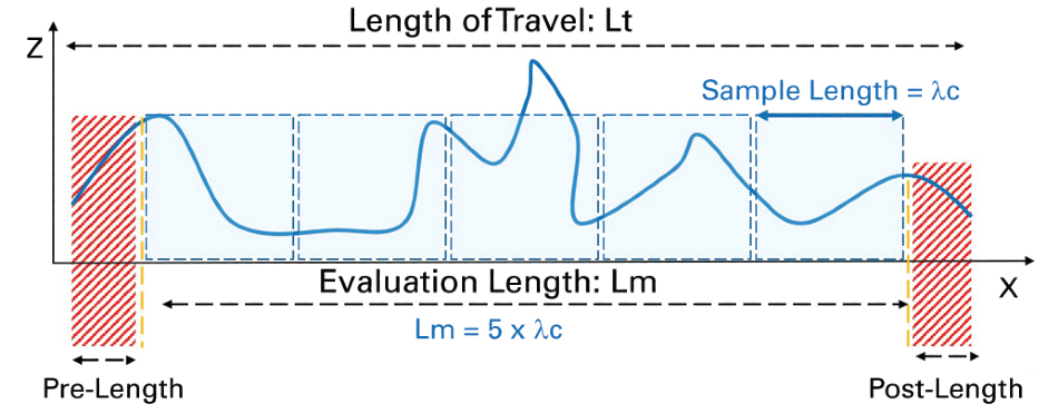
Figure 8. Details on total measurement length. Image Credit: Bruker Nano Surfaces

ISO 25178-2 is the sole standard for roughness calculation for areal measurement. This norm leaves the choice of evaluation length and cutoff values to the operator but dictates step-by-step filtering of the raw surface. Raw surface data gathered by the profiler first gets low-pass filtered (digital or spatial) to eradicate noise and outliers.

The result is the Primary Surface value. Most common spatial filters are based on Robust Gaussian or Gaussian Regression, which supplies a better response on sharp transitions and has almost no effect on borders.

Using shape removal, the Primary Surface is further processed to create the S-F Surface value. To remove waviness, an extra high-pass filter can be utilized to create an S-L Surface value. Users can crop borders further to acquire the scale-limited surface and work out roughness parameters.

The areal roughness standard does not distinguish parameters in these conditions: they are all labelled as S parameters. However, ISO 25178 does require listing the whole post-processing chain before displaying parameters, like cross-check control.

The same applies to roughness specifications on technical drawings, where exact measurement conditions have to be clearly labelled.

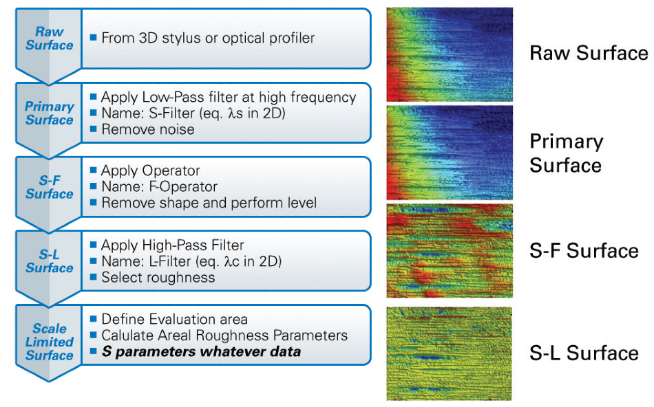
Figure 9. Step-by-step processing for areal roughness. Image Credit: Bruker Nano Surfaces

Measurement of Roughness Standard with WLI

Measuring sub-micron roughness and surface texture is one of the core applications of WLI-based profilers.

Its long-working distances and large field of view, combined with the method’s unique sub-nanometer vertical resolution, make it suitable for metrology of all precision engineered parts, ranging from forged flat metal to complex/curved surfaces, like gears or bore cylinders.

Further to this flexibility, the WLI optical profiler metrology capability benchmarks to certified roughness standards. Nine standards from three different manufacturers (Rubert,¹⁰ Halle,¹¹ NPL¹²) were investigated.

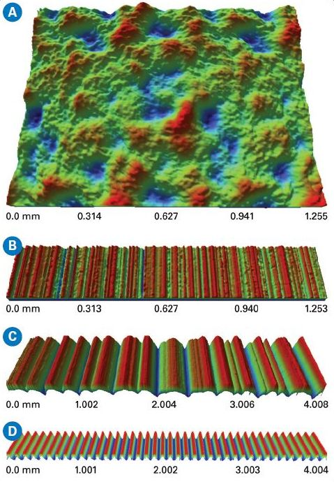
Figure 10. Topography rendered in 3D view of different roughness standards: (A) areal; (B-C) random profiles; and (D) sinusoidal profile. Image Credit: Bruker Nano Surfaces

The aim was to cover extensive vertical and lateral ranges in order to determine metrology capability over a larger amount of applications. This technique also provides comprehensive assessment for linearity performance over the vertical range.

In order to represent a real case for this native areal measurement technique, one areal artifact was also part of the evaluation.

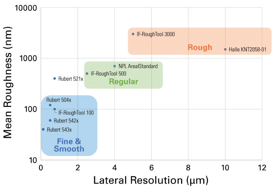
Figure 11. Plot of nominal mean roughness versus required lateral resolution. Image Credit: Bruker Nano Surfaces

Technical Considerations

Regular 1D roughness standards are designed primarily for stylus-based profilers. In that respect, lateral resolution capability is not dependent on scan length but instead on depth of the surface features and aspect ratio.

On the other hand, whenever a low-magnification objective is in use, an optical profiler has inherent changes in lateral resolution. So, it is vital to choose an objective which achieves a lateral resolution better than the λs cut-off.

To achieve the expected lateral resolution effectively, operators must also ensure that camera sampling is at least double the optical resolution. Otherwise, lateral resolution becomes limited by pixel size.

After the zoom lens and objective are properly selected, the evaluation length is ensured either by the stitching of multiple fields of view or by single acquisition. In this case, 5x, 20x, 50x, and 115x objectives were utilized.

The 115x objective was critical to resolve the finest patterns, while lower magnification (5x) was utilized for rougher surfaces that required less lateral resolution and longer evaluation length.

All data first underwent a 4th order polynomial removal before going through a Gaussian Regression band-pass filter. Cut-offs were chosen per the ISO 11562-1997 norm and settings from the standard certificate.

Final roughness extraction involved separating the areal image as a series of single-line profiles for which mean roughness (Ra) was calculated. Results not only indicated the average mean roughness along all profiles, but also showed fluctuation of the Ra value, one sigma deviation.

Measurements were repeated 30 times over each roughness standard in a fully static way, to address precision. This follows the recommendation from the Guide to the Expression of Uncertainty in Measurement (GUM).¹³ The overage factor k=2 was chosen, representing 95% of results for a purely random Gaussian distribution.

Results

Figure 12 shows a summary of all mean roughness results and plotting measured Ra value versus certified value in log-log scale. In examining the consistency and quality of the WLI optical profiler, there is great correlation over two decades, from over a micron to sub-100 nanometers mean roughness.

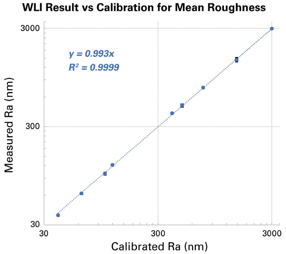
Figure 12. Measured mean roughness by WLI versus certified nominal value in log-log display. Image Credit: Bruker Nano Surfaces

For each result, error bars are represented utilizing ±2 dispersion from static repeatability. Yet, since, on average, they are below 1% of the result, they are hardly visible. This demonstrates how repeatable the WLI profiler is.

Further validation of results relies on the comparison between the confidence interval from the standard certificate and measurement of the dispersion interval. Figure 13 shows different configurations and specifies if a decision can be made from the data results.

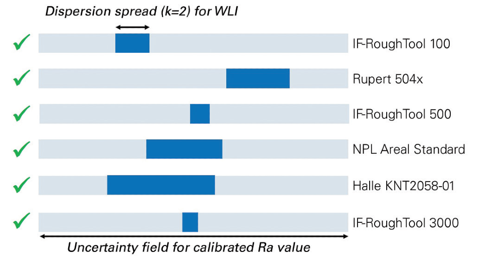
Figure 13. Mean roughness results assessment versus certification. Image Credit: Bruker Nano Surfaces

All of the results acquired with the WLI profiler are positively assessed, as the dispersion range always lies within the uncertainty of the standard. Data proves the accuracy of the WLI profiler measurements over the complete range of the available roughness standards.

Interestingly, the WLI profiler supplies reliable data at both extremes of the tested spectrum. On the rougher side, a low-magnification 5x objective enables precise measurement.

Combined with high-power illumination, robust algorithms for topography extraction from optical data provides a good ability to measure surfaces with rough, steady slopes. This extends the capability of the WLI profiler to tens of microns roughness, allowing the measurement of additive manufactured parts for instance.

At the other extreme, sub-micron fine pitch can be resolved clearly by a WLI profiler, giving adequate lateral resolution. By examining a direct comparison of WLI profiler measurements with those of an atomic force microscope (Dimension Icon, Bruker), this can be observed.

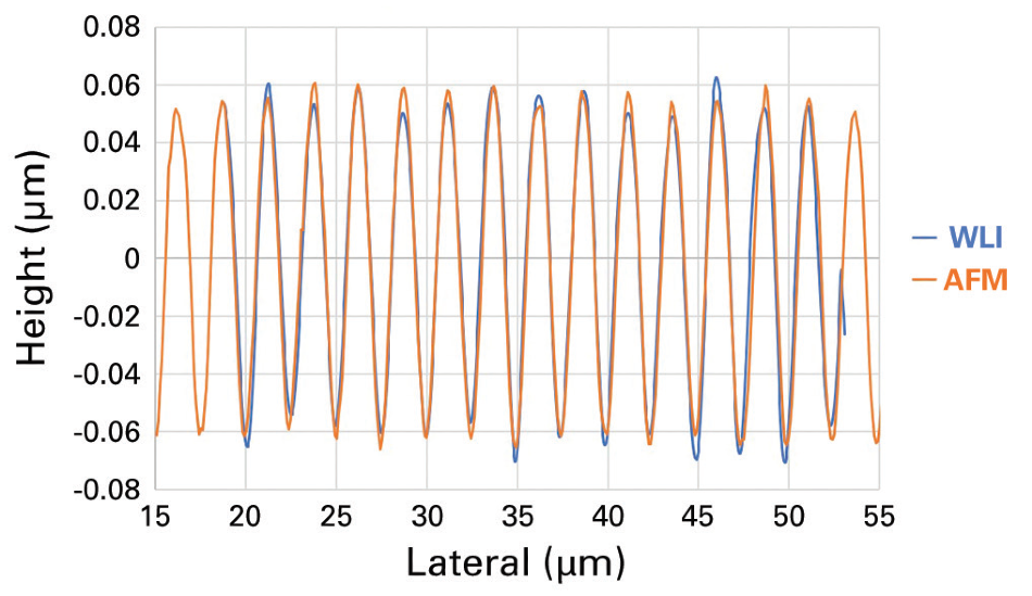
Figure 14. Profile comparison on sinusoidal standard between WLI optical profiler and AFM. Image Credit: Bruker Nano Surfaces

Figure 14 shows the correlation between section profiles made with the two methods. sub-nanometer vertical resolution and an advanced super-resolution algorithm, together with a high numerical aperture 115x objective, expand the transfer function of the optical profiler beyond micron lateral size.

Conclusions

This article has given a comprehensive overview on how surface roughness has evolved as a key manufacturing parameter, from method capabilities to normative guidance on both profile and areal measurements.

The WLI-based optical profiler measurement examples show perfect correlation with certified values when compared to certified roughness standards. With a dispersion range that is lower than 1% and a precise mean value the WLI profiler is capable of measuring mean roughness over 2 decades (from 3 µm to 40 nm).

WLI profilers also have a proven ability to measure steady, rough slopes, in addition to achieving sub-micron lateral resolution, all while maintaining vertical measurement that is extremely precise.

These factors demonstrate that WLI profiling will continue to play an integral part in the increasingly stringent R&D and manufacturing requirements for next generation industrial products.

Acknowledgments

Produced from materials originally authored by Samuel Lesko from Bruker Nano Surfaces. Special thanks to Reinhard Danzl and Franz Helmi from Bruker Alicona (Graz, Austria) for samples and review.

References

1. https://www.asme.org
2. https://www.iso.org/standard/22279.html
3. http://www.jsajis.org/index.php?main_page=product_ info&cPath=4&products_id=19626
4. https://www.iso.org/standard/74591.html
5. Seewig J (2005), Linear and robust Gaussian regression filters, J of Phys. 13:1:254-257.
6. Wyant J C (1995), Computerized interferometric measurement of surface microstructure, Proc. SPIE 2576:26-37.
7. Lange D A (1993), Analysis of surface roughness using confocal microscopy, J Mat Sc 28:3879-3884.
8. Bruker Alicona.
9. Novak E (2003), White-light Optical Profiler with Integrated Primary Standard, XVII IMEKO World Congress.
10. Rubert Profile Roughness Standards.
11. Halle Profile Roughness Standards.
12. NPL Areal Roughness Standards.
13. Guide to the expression of uncertainty in measurement

This information has been sourced, reviewed and adapted from materials provided by Bruker Nano Surfaces.

For more information on this source, please visit Bruker Nano Surfaces.