Some professionals working with particle counters believe it to be necessary to divide the particle counts of non-volumetric particle counters by the counting efficiency (CE) at the lower limit when establishing the “true” concentration of particles in the fluid system.
Others find it hard to grasp why two similar-sized channels of particle counters, albeit with varying limits of detection, fail to report the same value. This article discusses the science behind these differences and aims to allay any concerns associated with the characteristics of non-volumetric particle counters.
Definitions
- Counting Efficiency: A comparison between the percentage of particles identified in the fluid flow and the concentration of particles present.
- Instrument Sample Volume: The volume per unit time of fluid used for particle inspection.
- Instrument Flow Rate: The volume of fluid passing through the instrument measured in per units of time.
- Sample Volume Percentage: The remainder, expressed as a percentage, when dividing instrument sample volume by the instrument flow rate.
- Volumetric Particle Counter: A particle counter with 100 % sample volume.
- Non-Volumetric Particle Counter: Any particle counter where the sample volume percentage comes in under 100 %.
Background
The process of designing optical particle counters (OPCs) often involves making a compromise between increasing the signal coming from the particles and reducing the system’s noise generation. Typical sources of noise can include the light source itself, the optical components used for shaping the light, window surfaces/capillary walls, the sample fluid’s molecules, and the electronic circuits that collect and process the scattered light.
Particle counters with detection limits that exceed 100 nm are well-equipped when it comes to illuminating the sample cell walls while holding acceptable signal to noise (s:n) ratios. Due to their capacity to illuminate the complete sample cell with the uniform portion of the light source (usually a laser), these instruments are considered volumetric and offer a well-defined sample volume for the particles of interest.
Yet, when attempting to illuminate the sample cell walls in particle counters with detection limits below 100 nm, noise levels exceeding the amount of light collected from the particles of interest will be observed. To navigate this issue, the laser’s focus should be concentrated to a size smaller than the sample cell so to only inspect the region in the center of the cell for any particles. Concentrating the beam in this way generates a region of variable power density. With a beam smaller than the sample cell, particles are free to pass through the laser at any point over the cross-sectional area of the beam.
Some particles will pass through the center of the beam where the energy is most concentrated (Figure 1). These particles will yield a stronger signal and be recorded as a larger particle. The same sized particle which passes closer to the periphery of the laser beam, where the energy is considerably lower, will produce a weaker signal and be considered to be a smaller particle during measurement recording.
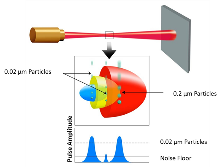
Figure 1. Sizing vs. Laser beam profile. Image Credit: Particle Measuring Systems
Particles gathered at the particle counter’s detection limit can only be identified when they pass through the center of the laser beam. Larger particles can produce a signal that is equal to a particle at the detection limit of the particle counter when passing through sections of the beam that are more distant from the center of the beam.
These particles will also be regarded as smaller sized particles during counting. The resulting outcome shows that the laser beam’s focal point is able to detect larger particles at a larger percentage during sizing and counting. Simply put, increases in particle size increase instrument sample volume. Particle Measuring Systems names this phenomenon “Sample Volume Growth.” All particle counters possessing instrument sample volume below 100 % of the instrument flow rate will demonstrate sample volume growth to some degree.
Discussion
At times the presence of sample volume growth (and any organic changes to counting efficiency with particle size) can prove to be an inconvenience for some users of particle counters, yet it is unfortunately unavoidable. The industry currently requires a particle counter that can identify particles as small as 20 nm and is pressing for one that can detect those at 10 nm or less.
Theis is where optical light scattering comes into its own as no other technology has proven itself to be as consistent, reliable, and capable of determining yield-limiting particle. Moreover, the phenomenon of sample volume growth is not a random factor that changes from instrument to instrument. It is influenced by the product’s design and all instruments made to follow that design will show very similar levels of sample volume growth.
A number of users make the decision to “correct for” first channel counting efficiency (CE) much lower than 100 %. This is achieved by dividing by the counting efficiency to determine a “real counts” number. It is crucial to understand that the lower detection limit CE is determined by introducing a known concentration of particles that correspond precisely to the size of the lower detection limit (i.e., 20 nm in the Example CE curve of Figure 2).
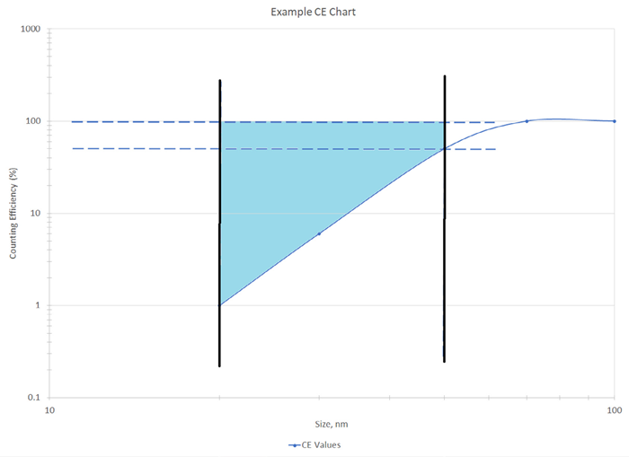
Figure 2. Ideal example counting efficiency chart. Image Credit: Particle Measuring Systems
The counting efficiency curve displayed in Figure 2 shows an idealized curve where the linear increase is approximated in relation to counting efficiency. The 20 nm channel in a particle counter will count all particles that range in size between 20 nm and 50 nm. Due to the fact counting efficiency scales across the channel with increases in particle size, dividing by the counting efficiency measured at 20 nm to determine the real counts of this channel would produce inaccurate results.
As shown in the chart in Figure 2, only the counts in the blue-shaded area are not reported. By forming a shape (triangle plus a rectangle) these “missing” counts are easily represented. The counts can be increased tenfold by correcting for the “missing” counts by dividing the reported counts by the 1st channel CE (1 % in this example). As exhibited in Figure 2, the “missing counts” are only on the order of ~4x in the less idealized version.
Since there is no way to easily characterize these real-world differences, establishing a correction factor that will work in all situations becomes increasingly difficult, even on the same fluid source. When faced with a difficult calculation of the absolute number of particles, the optical particle counter still offers actionable data representing changes in the system. For example, in an impending system failure (clogging filters, wear on a pump, etc.), proportional increases of the counts in this channel will give the user a good opportunity to respond to the situation before it becomes critical.
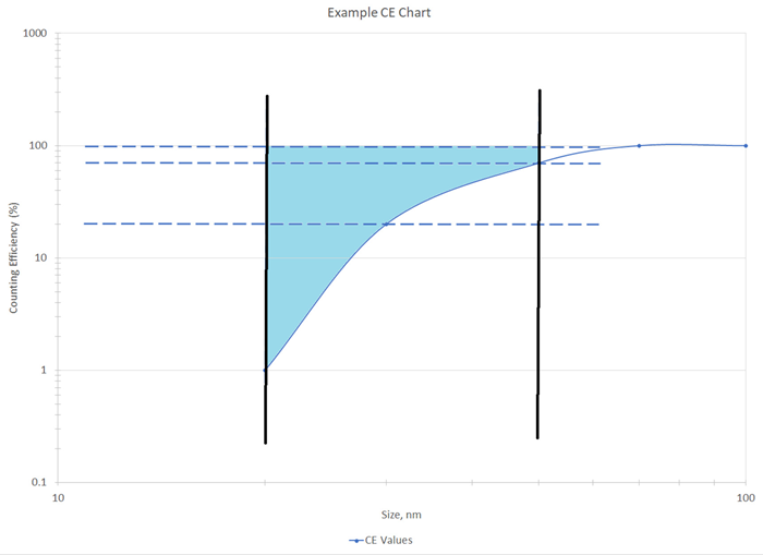
Figure 3. Real-world example counting efficiency chart. Image Credit: Particle Measuring Systems
Comparing Two Different Sensitivity Particle Counters
Many users question why an upper channel of a particle counter with greater sensitivity counts more particles than the first channel of a particle counter with a larger detection limit. This can be observed when comparing the UDI20 with the UDI-50 channels that sized particles greater than 50 nm. Obtaining an understanding of sample volume growth and the CE curve of these non-volumetric particle counters, it is obvious why there are differences between each of these instruments (Figure 4).
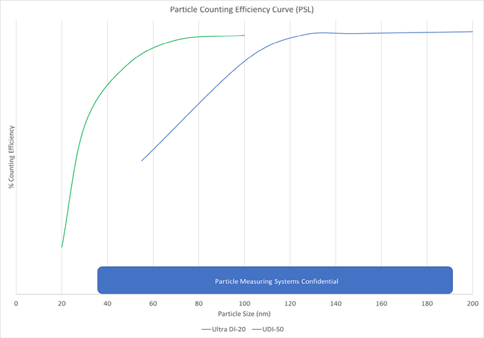
Figure 4. Particle counting efficiency curve comparison (UDI 20 VS UDI 50). Image Credit: Particle Measuring Systems
In Figure 4, the more sensitive UDI-20 particle counter is shown as it displays a much greater counting efficiency of particles >50 nm compared to the UDI-50 at equivalent sizes. Consequently, the UDI-20 should be able to count more particles than the UDI-50 in this size range. It should not be an issue that these two particle counters do not align in these channels.
The relationship between the data reported by each instrument remains consistent for any fluctuations in the system. For system contamination, the counts on both instruments at 50 nm should increase and when the system is purified (made cleaner) the counts on both should decrease. While a relationship between channels and relative system is preserved, by design, those particles are measured differently.
Summary
The semiconductor industry requires detection limits less than 100 nm while demanding a non-volumetric instrument design approach. All non-volumetric instruments demonstrate sample volume growth to some extent, which means a variable counting efficiency across the lower channel sizes and a lower counting efficiency at the lower limit of detection.
Variations in counting efficiency such as increases with particle size means the counting efficiency measured at a single particle size in this channel is not applicable across the entire channel. Applying counting efficiency as a correction factor does not yield “true” particle counts.
Particle counters with lower limits of detection, by design, will demonstrate a counting efficiency that varies at any given particle size channel when compared to a particle counter with a larger lower limit of detection. Yet, the fact these particle counters will exhibit different counts for any single particle channel, their trends remain the same.

This information has been sourced, reviewed, and adapted from materials provided by Particle Measuring Systems.
For more information on this source, please visit Particle Measuring Systems.