The most widely used methods for establishing particle size distribution are dynamic image analysis (DIA), sieve analysis, and static laser light scattering (SLS, also called laser diffraction). This article describes the benefits and drawbacks of each method, their comparability among each other as well as comprehensive application examples. Each technique comprises a characteristic size range within which measurement is possible. As illustrated in Figure 1, these partially overlap. The three techniques mentioned here, for instance, all measure particles in a range from 1 µm to 5 mm. However, the results for measuring the same sample can differ significantly.
This article will help to understand the informative value and importance of particle analysis results and to decide which technique is best suited for a certain application. The analyzers used for the measurements are image analysis systems CAMSIZER® P4 and CAMSIZER® X2 (Microtrac MRB), sieve shakers (Retsch), and laser diffraction size analyzer Horiba LA-960.
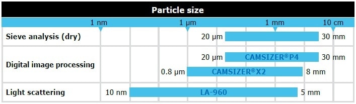
Figure 1. Measuring ranges of different methods
Sieve Analysis: Committed to Tradition
Sieve analysis continues to be the traditional and most widely used technique for particle size determination. A sieve stack contains a number of sieves with increasing aperture size stacked upon each other and the sample is positioned on the uppermost sieve. The stack is clamped to a sieve shaker and made to vibrate for a specific time period. Thus, the particles are distributed to the sieves in the stack (fractions) consistent with their size. Preferably, the particles pass the smallest possible sieve aperture with their smallest projection surface. Taking cubic particles as a model, this matches the edge length of the cube. For lenticular particles, the size established by sieve analysis would be a value between the diameter and the thickness of the lenses, as the particle is oriented diagonally towards the sieve aperture as seen in Figures 2 and 3. Hence, sieve analysis is a method which measures particles in their ideal orientation with a propensity to establish mostly the particle width.
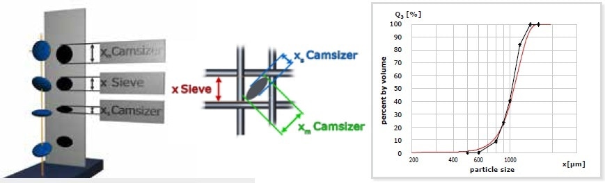
Figure 2. Model of a measurement of lenticular particles with sieve analysis and DIA. The lenses fall diagonally through the smallest possible sieve aperture. DIA “sees” the lenses larger or smaller, depending on its orientation. This results in different particle size distributions: the red curve shows the DIA result, the black curve represents sieve analysis results.
Sieve analysis is performed up to a point where the sample mass on the individual sieves no longer varies (= constant mass). Each sieve is weighed and the volume of each fraction is calculated in percent by weight, providing a mass-related distribution. The resolution of sieve analysis is restricted by the number of obtainable size fractions. A standard sieve stack accommodates a maximum of eight sieves which means that the particle size distribution is based on just eight data points. Automation of the process is not possible which makes it quite time-consuming. The single steps of sieve analysis are: initial weighing, 5 to 10 minutes sieving, back weighing, and cleaning of the sieves. The most frequent sources of error are: old, worn or damaged sieves (too fine results); overloading of the sieves (blocking of sieve apertures, too coarse results); or errors in data transfer. It should also be taken into consideration that the aperture sizes of new standard-compliant sieves are also subject to specific tolerances. The average real aperture size of a 1 mm sieve, for instance, is allowed to deviate around ±30 µm, for a 100 µm sieve, it is ±5 µm (i.e. the average real aperture size falls between 95 and 105 µm). However, this is only the mean value which indicates that a few of the apertures can be even larger. With adequate sieving time, the particles locate the largest apertures which results in particles larger than the nominal aperture size of the sieve passing through. Hence, the sieve becomes effectively larger than the nominal aperture size implies. These tolerances are mainly apparent in sieve analysis results of samples with a narrow particle size distribution or of spherical samples, as can be seen in Figure 4 which illustrates the measurement results of a sample of glass beads.
Besides the dry sieving process with wire mesh sieves explained in this article, there are other special techniques such as air jet sieving or wet sieving.
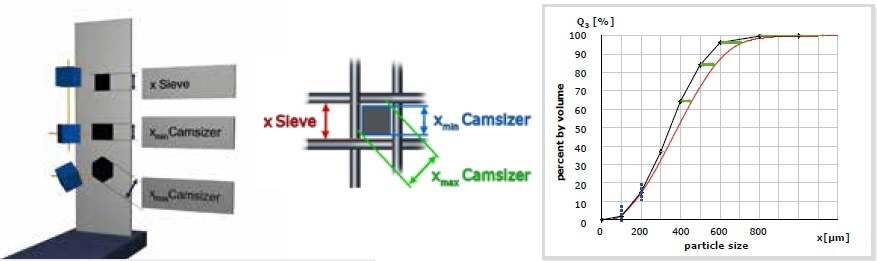
Figure 3. Model of a measurement of cubic particles with sieve analysis and DIA. Sieve analysis determines the edge length whereas DIA measures the edge length or, depending on the orientation of the particle, a higher value (max. edge length * square root of 2 of the hexagonal projection), but never smaller than the value obtained by sieve analysis. Red curve = measurement with DIA, black curve = sieve analysis.
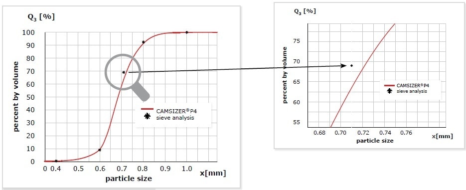
Figure 4. Measurement of a glass bead sample with DIA (CAMSIZER® P4, red) and sieve analysis (* black). The measurements can only be compared at the points which represent the sieve fractions. There is excellent agreement between the results. When taking a closer look at the data at 710 µm, it is apparent that the deviation of the Q3(x) value is 6% which seems quite a lot at first sight. However, the deviation in size is only 13 µm and is thus within the tolerance of a 710 µm sieve which is ±25 µm. As the cumulative curve is very steep at this point, even a small difference in size has a strong impact on the Q3(x) value.
Dynamic Image Analysis (DIA): What You See Is What You Get
For particle characterization, there are two methods of image analysis. Static image analysis is essentially a microscope which measures the sample positioned on an object slide step by step. Although the quality of the images is excellent and the optical resolution quite high, this technique has a few decisive disadvantages with respect to representing particle size distributions: the size range is restricted, the process is quite time-consuming, and the quantity of analyzed particles is usually not enough to provide a statistically sound statement regarding the total sample. Therefore, only dynamic image analysis will be discussed in this article. This method includes a flow of particles passing a camera system in front of an illuminated background. Figure 5 illustrates a schematic of this measurement principle as implemented in the CAMSIZER® X2. The system measures free falling particles and suspensions, and also features dispersion by air pressure for those particles which are inclined to agglomerate. Advanced DIA systems analyze over 300 images per second in real time, detecting millions of individual particles in just a few minutes. This performance is based on rapid cameras, short exposure times, bright light sources, and powerful software.
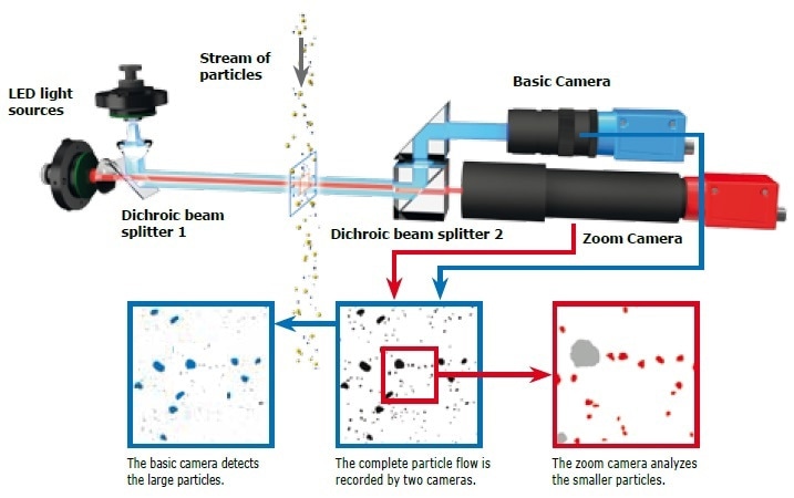
Figure 5. The image analysis system of the CAMSIZER® X2. The CAMSIZER® series uses patented dual camera technology with different resolutions to realize an extremely wide measuring range. The cameras capture the projections of the particles.
Contrary to sieve analysis, DIA measures the particles in a fully random orientation. A wide range of size and shape parameters are measured based on the particle images. For instance, typical size parameters are length, breadth, and diameter of equivalent circle (Figure 6). The particle shape parameters include convexity, sphericity, symmetry, and aspect ratio. The key feature of DIA is the extremely high detection sensitivity for oversized grains. For instance, the CAMSIZER® P4 is designed to detect each single particle of a sample and the model CAMSIZER® X2 has a 0.1% detection limit for oversize particles. The resolution of dynamic image analysis systems is simply unbeatable: smallest size differences in the micrometer range are detected reliably and multimodal distributions are determined without fail.
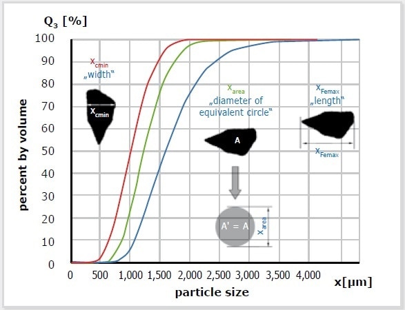
Figure 6. DIA uses various size definitions to determine the particle size distribution. Consequently, one measurement can produce several distributions. In this example, the red curve is based on the measurement of particle width; the blue one represents particle length. The parameter X-area stands for the diameter of equivalent circle which is defined as the particle size. It depends on the original question which results are finally relevant. When examining fibers or extrudates, the length parameters are of interest; width is more important if comparison to sieve analysis is required.
The particle “width” is the common parameter if DIA is compared to sieve analysis. However, while measuring irregularly shaped particles, still there are systematic differences in the achieved results because the particles are measured by DIA in random orientation. Figures 2 and 3 show how the differences in the particle size measurement occur and how they can be interpreted. For each defined particle shape, the differences in particle size distributions are very systematic. The CAMSIZER® software includes algorithms that allow users to correlate the DIA results to those achieved by sieve analysis with a 100% match (Figure 7). This process is commonly used in particle size analysis applications for quality control because many products are analyzed by various laboratories with different measuring techniques in a globalized market, creating a need for comparability.
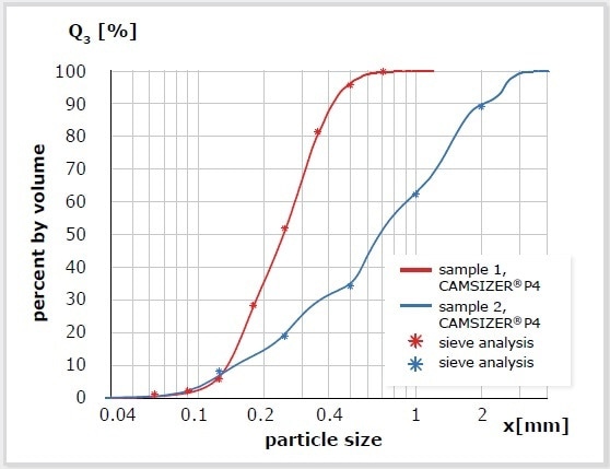
Figure 7. Example for the excellent agreement between measurement results of two sand samples obtained by DIA (red and blue curve) and sieve analysis (*).
Laser Diffraction: Spheres and Collectives
Using static laser light analysis, also known as laser diffraction, particle size is indirectly measured by detecting intensity distributions of laser light scattered by particles at various angles. The setup of an advanced laser granulometer, such as Horiba’s LA-960, is shown in Figure 8. This method is based on the fact that light is scattered by particles and the correlation between particle size and intensity distribution is well-known.
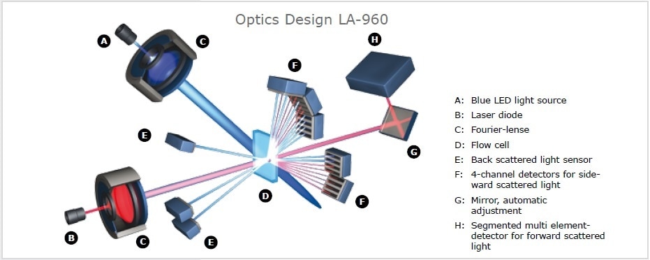
Figure 8. The laser light scattering spectrometer Horiba LA-960 uses two light sources and 93 measurement channels to record the scattered light pattern over a wide angle. It is possible to analyze suspensions, emulsions as well as dry powders in a measuring range from 0.01 m to 5,000 µm.
In other words, large particles scatter the light to small angles, while small particles generate large-angle scattering patterns. When large particles generate rather sharp intensity distributions with typical maxima and minima at defined angles, small particles’ light scattering pattern becomes increasingly diffuse and thus overall intensity decreases. In a polydisperse sample, it is very difficult to measure differently sized particles because the particles’ individual light scattering signals superimpose each other.
Static laser light scattering (SLS) is an indirect method that determines particle size distributions due to the superimposed scattered light patterns produced by a whole collective of particles. Algorithms are based on MIE theory with the assumption that particles are optical and spherical characteristics such as absorption index (AI) and refraction index (RI) are well known. A great benefit of SLS is the extremely wide measuring range; no other methods presented here is capable of reliably detecting particles smaller than 1 micron. SLS analyses are easy to perform and they can be automated to a great extent. A disadvantage of this method is its relatively poor resolution. If the amount is below 2 Vol%, even the most recent analyzer generation cannot detect oversized fractions. In order to resolve multimodal distributions, the size of the two components involved has to differ at least by factor 3. More than three different components are basically not detectable in a mixture. The example of a mixture of polystyrene-latex standard particles is shown in Figure 9. Contrary to SLS, dynamic image analysis is able to detect exactly four different particle sizes while the laser diffraction analyzer cannot accurately resolve the 10 µm and 12 µm particles.
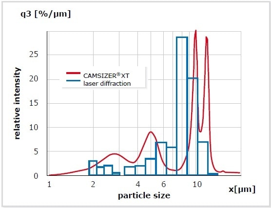
Figure 9. Measurement of a mixture of four particle standards (2.5 µm – 5 m – 10 µm – 12 µm). While DIA is able to distinguish the four components (red), laser diffraction identifies only three.
The comparability between DIA, SLS, and sieve analysis using the example of ground coffee is illustrated in Figure 10. Sieve analysis offers the best results; the particle breadth measurement using the CAMSIZER® X2 comes very close to this. There is no clear comparability between laser diffraction and sieve analysis; the result achieved with SLS corresponds approximately to the X-area parameter (diameter of equivalent circle). The different particle dimensions that are measured are all attributed to particles that are spherically shaped. Therefore, SLS provides broader size distributions than image analysis at all times.
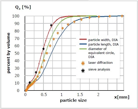
Figure 10. Measurement of ground coffee with different methods. DIA, particle width (red); DIA, particle length (blue); DIA, diameter of the equivalent circle (green); laser diffraction (orange *); sieve analyses (black *).
This is even clearer in Figure 11 which illustrates a comparison of the measurement of cellulose fibers. DIA distinguishes between the length and thickness of the fibers, whereas SLS is not able to do so. The laser diffraction measurement curve first runs parallel to the width measurement of DIA (red) and after that approaches the “fiber length” (blue). The laser scattering result includes length and width information, and all are merged into one size distribution.
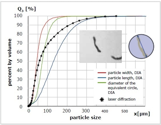
Figure 11. Measurement of cellulose fibers. The CAMSIZER® XT (image analysis) measures particle breadth (red), particle length (blue), and X-area (green). The SLS measurement (*) is a mixture of breadth and length and shows a continuous transition. DIA can distinguish between breadth and length.
Conclusion
Among all the methods discussed in this article, dynamic image analysis is the only method that is capable of providing precise information about the particle size while also taking into account their shape. This means that, if required, it is possible to follow the results achieved by other methods and compare them. The information content and resolution of DIA are much superior to sieve analysis and laser diffraction, thanks to the direct measurement of particles.
The benefits of sieve analysis are the wide usage and the comparatively cost-efficient equipment.
Using laser diffraction for particle size analysis is the only method that allows for measuring sizes smaller than 1 micron.
Table 1 and 2 summarize both the advantages and disadvantages of the respective method.
Table 1. Comparison sieve analysis and dynamic image analysis
| |
Sieve Analysis |
Image Analysis |
| Measuring range |
20 µm – 125 mm |
CAMSIZER® P4: 20 µm – 30 mm
CAMSIZER® X2: 0.8 µm – 8 mm |
| Particle shape analysis |
no |
yes |
| Detection of oversized grains |
each particle |
CAMSIZER® P4: each particle
CAMSIZER® X2: < 0.01% Vol. |
| Resolution |
poor |
very high |
| Dissolution of multimodalities |
poor |
excellent |
| Repeatability and lab-to-lab comparison |
limited |
very good |
| Comparability of methods |
identical results possible |
| Handling |
simple, time-consuming, error-prone |
simple, objective, fast |
Table 2. Comparison laser diffraction and dynamic image analysis
| |
Laser Diffraction |
Image Analysis |
| Measuring range |
10 nm – 5 mm |
> 0.8 µm |
| Particle shape analysis |
no |
yes |
| Detection of oversized grains |
> 2% |
CAMSIZER® P4: each particle
CAMSIZER® X2: < 0.01% Vol. |
| Resolution |
good in the micron range, getting worse with increasing particle size |
excellent over the whole measuring range |
| Dissolution of multimodalities |
limited (starting with factor 3 for mixtures) |
significantly better size resolution |
| Comparability to sieve analysis |
poor |
identical results possible |
| Information content |
equivalent diameter, spherical model, indirect method |
real particle dimensions, direct length |

This information has been sourced, reviewed and adapted from materials provided by Microtrac MRB.
For more information on this source, please visit Microtrac MRB.