Dynamic Image Analysis (DIA) has become a widely used method for the routine analysis of the size and shape of particles within numerous industries. This article will explain how DIA successfully replaces traditional sieve analysis techniques to produce results that are extremely close to the product specifications that have originally derived from sieve techniques. Industry users that utilize DIA benefit from a reduced workload, higher sample throughput and more detailed measurement results.
While still a standard and cost-efficient method for the routine determination of particle size distributions of both powders and granulates, sieve analysis can also be prone to error and subject to various inaccuracies. For example, the time that is required to complete a single analysis may add up to 15 -30 minutes of work involving weighing, sieving process and cleaning.
The information obtained by this method is limited, as the number of data points is directly related to the number of test sieves that are available. In contrast, DIA delivers high-resolution measurement results within 2 - 3 minutes , and simultaneously provides information on the particle shape.
When comparing these two analysis techniques, some systematic differences can be observed in the results that are generated. These are discussed in the following paragraphs by comparing the results generated by DIA and sieve analysis in various application examples for different materials and particle shapes. Possible solutions on how to overcome these deviations and establish a robust and reliable correlation of DIA and sieve data will also be discussed in this article.
Measurement Principles of DIA and Sieve Analysis
The measurement principle of dynamic image analysis involves the use of both a strong LED light source that illuminates a flow of particles and a camera system that captures images of the particles in the form of shadow projections. These images are then transferred to a PC that is equipped with a powerful evaluation software which processes the data to generate the various size and shape distributions.
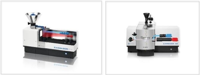
Figure 1. Two high-end DIA particle analyzers: CAMSIZER P4 (left) and CAMSIZER X2 (right) from Microtrac MRB. The P4 model is suitable for fast analysis of pourable bulk solids in a size range from 20 μm to 30 mm. The X2 model is optimized for fine powders in a size range from 0.8 μm to 8 mm.
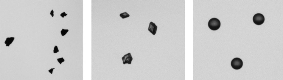
Figure 2. Example images from CAMSIZER measurements: activated carbon (left), sugar crystals (middle), and expandable polystyrene beads (right).
Figure 1 shows two of Microtrac MRB’s state-of-the-art image analyzers, CAMSIZER P4 and CAMSIZER X2, both of which are capable of recording and evaluating 60 or 320 images per second, respectively. The results generated by these analyzers are based on the size and shape data acquired from hundreds of thousands, or even millions of individual particles, depending on the particle size and sample quantity..
An unambiguous definition of particle size only exists for spherical particles, whereas the particle size for all other particle shapes may be derived from different physical dimensions.
Figure 2 shows the different size definitions that are used for the 2D projection of an angular particle: width (xc min, smallest chord); length (xFe max, maximum length); equal area diameter (xarea). Which definition is used will determine what type of results are achieved. While each particle distribution is correct, they will all provide information on different sample properties.
For example, users who want to correlate image analysis with sieving results will use the size definition xc min, since the particles will preferentially pass through a sieve mesh with their smallest projection area that corresponds to the width of the particle, as demonstrated in Figure 2.
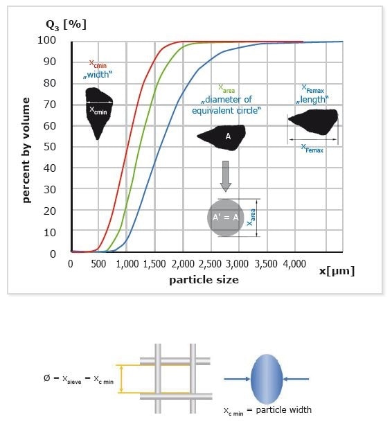
Figure 3. Size definitions used in dynamic image analysis. The parameter xc min (particle width) provides best correlation with sieve results.
DIA and Sieve Analysis of Spherical Particles
Spherical particles are the easiest example that can be used to compare the different sizing techniques, as there is only one possible particle diameter, regardless of the orientation, so any notable deviations are unlikely.
Some examples of relatively round particles include pellets that are formed during granulation and coating processes, glass beads, EPS particles and certain metal powders. As shown in Figure 3, the measurement example presents a divergence between the CAMSIZER result, (size definition xc min) , and the sieve analysis results which seems to be finer.
Each analytical test sieve is manufactured and inspected according to the standard ISO 3310-1, which defines how much the real apertures of a test sieve are allowed to deviate from the nominal aperture sizeThe mean aperture size and standard deviation are examined individually for both directions, which are referred to as the warp and weft of the wire mesh, as well as the maximum allowed opening.
The tolerance allowed for a 500 μm test sieve is ±16.2 μm for the mean real aperture and the maximum allowed aperture is 580.5 μm. Consequently, each ISO 3310-1 compliant test sieve will feature a significant number of openings that are larger than the nominal size, even if the mean aperture is close to the nominal size.
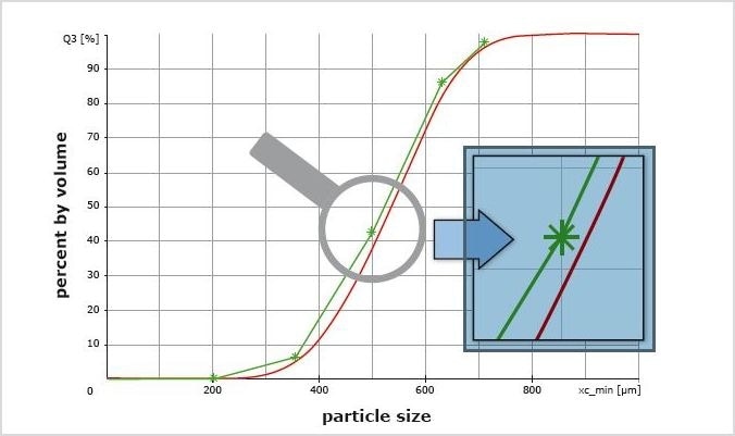
Figure 4. Sieve analysis (green *) and CAMSIZER P4 result (red) for round particles, cumulative distribution Q3. The offset is only a few micrometers and well within the tolerance of the test sieves. As the distribution is very narrow (sharp increase of the Q3 curve), a small deviation in size of only 15 μm results in a large difference in Q3 of almost 5 %.
As a result, large particles that should be retained, are able to pass the sieve and will therefore be classified as finer than they actually are. Hence, the resulting sieve data is less accurate than the CAMSIZER result, as this method is capable of accurately determining the size of the spherical particles. The magnitude of this deviation depends on how much the individual sieves deviate from the nominal size.
As shown in Figure 4, this information can be obtained from the calibration certificate of each test sieve that is supplied by the manufacturer upon request. To achieve an accurate correlation between DIA and sieve analysis results, it is recommended to consider the real aperture size from the calibration certificate. If this is not possible, the user can also utilize a constant factor that can be determined for each particle size to compensate for the effect of the sieve tolerance.
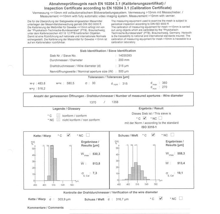
Figure 5. Excerpt from a calibration certificate of a 500 μm analytical test sieve. The mean real aperture is 513.8 μm and 513.4 μm respectively. The maximum aperture is 558.3 μm and 530.3 μm respectively. This sieve complies with ISO 3310-1 but allows round particles as big as 530 μm to pass.
It is commonly observed that sieve results change when one test sieve is exchanged for another with the same nominal size. Consequently, the correlation factor to DIA is only valid if the sieves are not changed.
DIA and Sieve Analysis of Non-Spherical Particles
Some systematic differences exist between the results obtained by DIA and sieve analysis which arise from the particle shape.
Angular Particles
Sieve analysis determines the edge length of the cubes and is therefore a measurement technique which determines the particle size in a preferred orientation. During the sieving process, particles have the opportunity to compare themselves with different apertures in different orientations.
For example, as shown in Figure 5, cubical-shaped model particlespass the smallest possible aperture with their smallest projection area. This does not occur when DIA is used, as this this technique captures the particles in absolutely random orientations.
For some of these random 2D-orientations, xc min has been shown to produce the same numerical results as when sieve analysis is used, with the cube face pointing towards the camera). In many cases, the xc min of the random 2D particle projection will produce a larger numerical value than that obtained by sieve analysis.
The largest possible value is reached when the corner of the cube is pointing towards the camera. Then the 2D projection is a hexagon with an xc min that is equal to the edge length (d) times square root of two, as shown in the following equation:
xc min = d · √2
The DIA system can therefore measure a cuboidal particle that is up to 1.414 times larger than it would be possible with sieve analysis. Consequently, the correlation between DIA and sieve analysis for real angular particles is usually good for the fine fraction of the distribution because the small particle projections are captured. The coarse fraction, however, exhibits a worse comparability because it represents the larger projection areas.
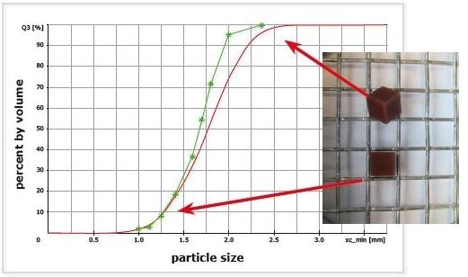
Figure 6. Sieve analysis (green *) and CAMSIZER P4 result (red) for angular, approximately cubicalshaped particles. Cumulative distributions Q3.
Flat, Flaky and Lenticular Particles
Flaky or lenticular particles are also able to pass through the smallest possible sieve aperture with their smallest projection area. They will, however, orientate diagonally in the square holes of the sieve, so that the numerical value obtained from sieving is a value between the thickness and diameter of the particle as can be seen in Figure 6.
In a random orientation, the measured xc min value of the flaky particles will typically lie between the specific thickness and diameter of the particle, hence the result can be either larger or smaller than that obtained by sieve analysis.
For real samples, this will cause an intersection between the cumulative curves. The distribution of these particles measured by image analysis will typically remain wider than the distribution data obtained from sieve analysis.
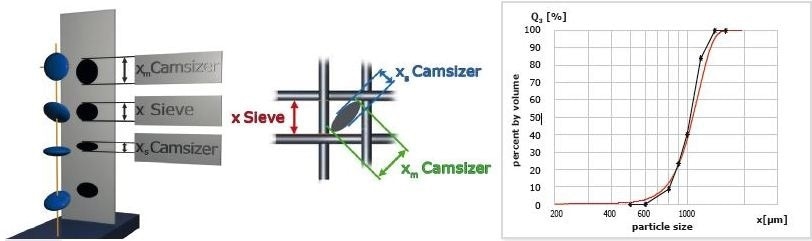
Figure 7. Sieve analysis (black *) and CAMSIZER P4 result (red) for flattened particles, cumulative distribution Q3. Particles are passing the apertures diagonally, the CAMSIZER can measure a smaller or larger size depending on the orientation of the particle during detection. The resulting distribution is therefore wider than the sieve analysis result.
Influence of Distribution Width and Sieve Correlation
From these observations it is clear that a simple “shape factor“ that will shift the entire distribution by a constant factor, can never be enough to obtain full compliance between sieve analysis and DIA. A more promising approach is the use of different factors that depend on the Q3 value. This method can be applied for all samples with the same shape and width of distribution. If the distribution width changes, however, this correlation technique will fail as well as the deviations between DIA and sieving also change with the distribution width.
Consider a sample of lenticular particles as in Fig. 6. A real sample will contain lenses of different sizes and due to orientation effects, some of the large ones will be detected as “too small “, and some of the small ones will be detected as “too large” by the image analyzer. For a wide distribution with lenses of many different sizes, these deviations will cancel each other out and the overall correlation will be very good.
However, if all lenses have identical thickness and diameter, the systematic differences between the two techniques become apparent. Thus, for narrow distributions, a stronger correlation factor is required than for wide distributions. In practice, users who deal with wide distributions often don’t need to apply any correlation mechanism.
For all other cases, it is possible to achieve a strong correlation that is valid for all particles with a particular shape but is independent of width of distribution. The idea is to let the image analyzer measure a test sample of a specific material where the deviation from sieving is highest, and that would be a very narrow distribution.
From this result the algorithm will learn the fundamental difference for this material, independent from distribution width and can apply this to any other sample with similar particle shape. This training sample is obtained by sieve analysis; the narrower the fraction, the better the correlation algorithm, e. g. 600 µm – 630 µm or 1.12 mm – 1.18 mm, this will produce particles that are all the same size in terms of sieving.
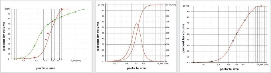
Figure 8. leftz: Size analysis of two sand samples, one with a wide distribution (Sample 1, green) and one with a narrow distribution (Sample 2, red). CAMSIZER P4 results and corresponding sieve data as *. The wide distribution is in much better agreement with sieving, the red curve shows the typical deviations. Middle: CAMSIZER P4 analysis of the fraction 450 μm – 500 μm of sample 2. This fraction is suitable as a training sample to find a correlation function. If this correlation is then applied to the measurement result of sample 2, DIA and sieve analysis match perfectly (right).
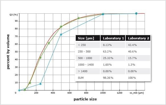
Figure 9. Example of a faulty sieve analysis. Results of a fine sand sample: CAMSIZER P4 (red). Sieve results from two different laboratories: Lab 1 (blue *), Lab 2 (green *). The result of Lab 1 is significantly coarser than those of Lab 2 and of DIA. Too much initial sample weight leads to overloading of the 250 μm and 500 μm sieves and small particles don’t have the opportunity to pass. Furthermore, the fractions do not add up to 100% for the analysis of Lab 1 (loss of sample!). The sieve result of Lab 2 is correct and in good agreement with DIA.
With the previously described procedure, the user of a CAMSIZER system can find a strong sieve correlation in three simple steps:
- CAMSIZER analysis
- Sieve analysis
- CAMSIZER analysis of a narrow fraction
The basic requirement for successful sieve correlation is, however, that the sieve data is correct. It is not possible to match DIA data with faulty sieve analysis results, so always make sure that the test sieves used are in good condition and are clean.
Damaged or worn out sieves must be replaced. The sieving process has to be long enough to give all particles the opportunity to pass, which means the sieving process has to be continued until the mass of sample on any sieve does not change with prolonged sieving time.A frequent error in sieve analysis is overloading. If too much sample is placed on one sieve, apertures will be blocked, preventing small particles from passing. The smaller the particle size, the less sample is allowed.
Some users always take 100 g of sample, because then gram equals percent and the calculation is much easier. For many fine samples 100 g is already too much, plus there is always the danger of making a sampling error when a particular mass is used. It is better to reduce the sample amount with a sample splitter and use one aliquot for the analysis.
Conclusion
Dynamic Image Analysis is a very precise and reliable technique for the characterization of particle size and shape of bulk solids. In comparison to traditional sieve analysis it offers a reduction of workload and higher throughput plus much additional information on the material at hand.
Due to the sophisticated material-specific correlation functions that can easily be established by the user it is possible to achieve results that match sieve analysis very accurately and reliably. When interpreting the results, the limitations and inaccuracies of sieve analysis have to be taken into consideration.
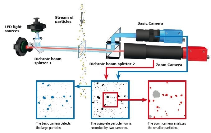
CAMSIZER Dual Camera Technology

This information has been sourced, reviewed and adapted from materials provided by Microtrac MRB.
For more information on this source, please visit Microtrac MRB.