Using FlexiSpot to Improve the Precision of the Quantification of Non-Homogeneous Samples

Quantitative Micro-XRF analysis incorporates data across the whole irradiated and detected sample area. The quantification method requires a homogeneous sample to properly determine its composition. Most non-manufactured samples, however, such as geological examples, are heterogeneous and their components are not as consistently distributed as mass-produced samples such as can be seen in prefabricated steel or glass.

Historical XRF analysis requires substantial preparation to attain sample homogeneity. By using spatially resolved Micro-XRF an additional advantage is gained meaning that little or no sample preparation is necessary.

Performing analysis with spatial resolution at the micrometer scale can mean it is difficult to find points where the quantitative results are representative of the whole sample or, indeed, a specified partial sample area.

Powders and milled samples are classic examples of homogeneity at the millimeter scale, but can display large point-to-point variation if measured at tens of micrometers resolution.

M4 TORNADO’s FlexiSpot feature allows large area investigation with a micrometer resolution: Samples can be measured with a spot size of <20 µm and also with an added spot size of a few 100 µm. The larger irradiated spot permits more accurate quantification of non-homogeneous samples or samples with irregular surfaces, such as powders, since data is combined in the analysis across the increased detection area.  

Functional Principle

The polycapillary lens in the M4 TORNADO generates a convergent X-ray beam to focus the radiation of X-ray tube. The plane in which the beam waist occurs is known as the focal plane. The beam width at this point is <20 µm for Mo Kα (sample fluorescence).

The FlexiSpot feature is based on the X-ray beam being wider both above and below its focal plane. By adjusting the sample into an “out-of-focus” situation, the irradiated area is larger. Considering the common beam divergence of polycapillary lenses, spot sizes of 100–200 µm can be attained by shifting the sample about 2–3 mm out of the focal plane (see Fig. 1).

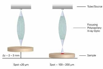
Figure 1. Functional principle of generating a variable spot size

Sample Preparation

The sample being analyzed in this case was clay obtained from the Cretaceous-Paleogene-boundary in Petriccio, Italy. The clay was pulverized and consequently compressed into a pellet using 20 % binder material. This is a well-used method of preparation and it yields decent quality homogeneous material for traditional XRF analysis. However, this case demonstrates that in a light microscope with 100x magnification, the obtained image of the sample shows that at a 10 micrometer scale the sample is not nearly as homogeneous as previously thought. Fig. 2 shows the clay pellet sample with two different spot sizes.

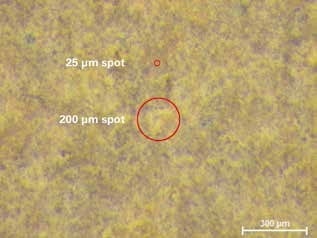
Figure 2. Clay sample in 100x magnification showing obvious inhomogeneity. The red circles indicate the set excitation spot diameters of 20µm and 200µm.

Measurement Conditions

Measurements were executed with a Bruker M4 TORNADO equipped with a Rh X-ray tube and a polycapillary lens. This setup has high spatial resolution with fast data processing and a mechanical high-speed X-Y-Z stage for locating the sample and performing distribution analysis. The following standard measurement configuration was provided for the setting up of the system:

• Tube voltage of 50 kV
• Current of 200 µA  
• No primary beam filter
• Chamber pressure of 20 mbar.

Spatially resolved quantitative analysis on a heterogeneous sample was performed on multiple points to attain an illustrative value for the entire area. The mean quantitative results are then considered as the “correct” result. The reliability of the result is specified by the standard deviation of the different results. For the small analysis spots the standard deviation was very high and accordingly the results may be statistically correct or not meet set criteria.

Using the Multi-Point workspace of the M4 TORNADO software, this method used six arbitrary positions which were defined to take measurements using spot sizes of both 20 µm and 200 µm, respectively (see Fig. 3a–b). To obtain decent statistics for the light and minor elements, the collected single point measurement time was set to 120 s.

Using the same excitation settings, a 40 mm x 40 mm segment of the model sample was then mapped with 50 µm pixel size over an acquisition time of 4 ms per pixel. To attain the comparable inclusive measurement time of 120 s in the same way as the point measurements, six areas of 75 mm² were extracted from the acquired HyperMap data cube (see Fig. 3c).

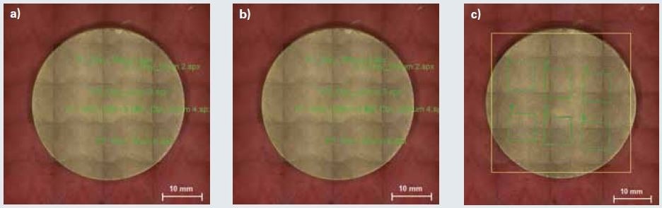
Figure 3. Mosaic image of the sample with defined measurement positions and areas

Results

Table 1 gives a summary of the quantification results for six different measurement positions, each obtained with a spot size of 20 µm and 200 µm, and six mapping areas, respectively. The standard deviation for the measured compositions diminishes with bigger analyzed sample surface area, while the calculated concentrations go on continuing to be stable.

Fig. 4 shows this tendency for the oxides of the main elements SiO₂, CaO, Fe₂O₃, and Al₂O₃. The mean and sigma values for the 75 mm² areas are representative for the sample with preset measurement conditions. With reduced study areas, the deviations of the quantified values come to be larger while the “correct” value is now inside the range of obtained uncertainties.

Table 1 and Fig. 4 show that the increased spot size of 200 µm promotes enhancement of the differences by a factor of 2 or better in comparison to the regular spot size of 20 µm. It should be noted that this condition relates to an equal measurement time.

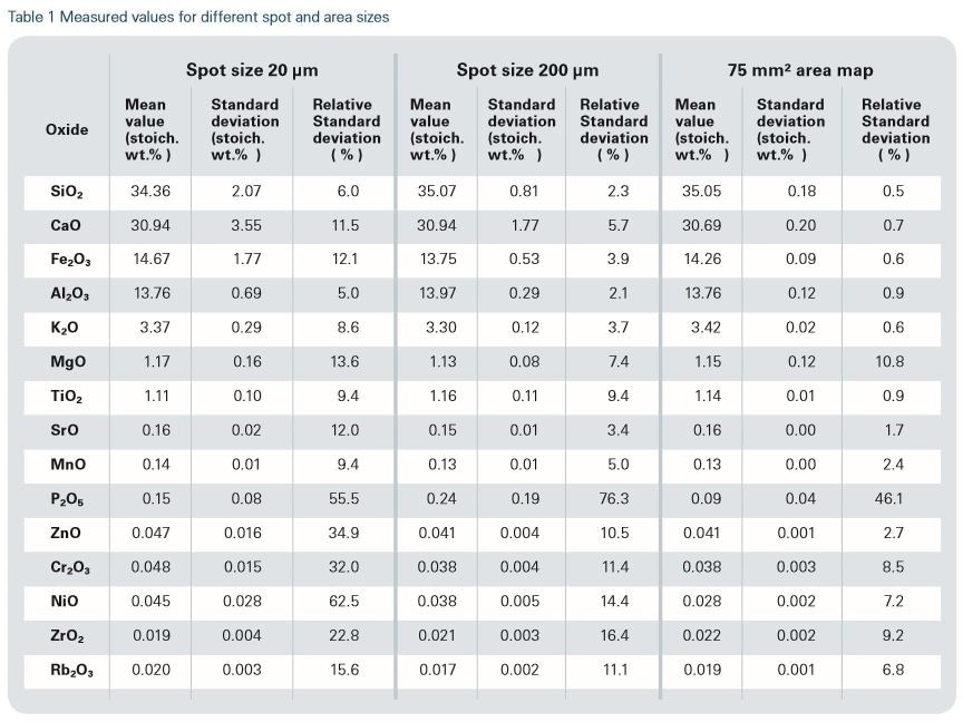
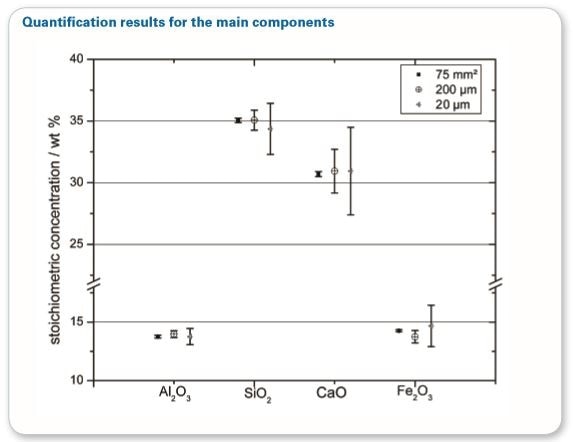
Figure 4. Quantified values for the main matrix components with two sigma standard deviation (as obtained from six measurements

The graph in Fig. 4 suggests that only a full area map can provide dependable results, it should be realized that the time taken to acquire data in this area is 5 times greater than the acquisition time for the multipoint measurements (1:04 h in comparison to 12 min). For the majority of applications, the deviations resulting from the point spectra measurements are fully satisfactory.

Only the results of Mg and P, which are both low concentration light elements, do not follow the strict trend. This variation is a result of the inhomogeneity and lower measurement statistics of these characteristic fluorescence lines.

Conclusion

The comparison of measurements taken using a variation of spot sizes and areas plainly displays an important enhancement of the relative standard deviations when bigger areas are analyzed using M4 TORNADO’s FlexiSpot. However, point measurements with a spot size of 200 µm do deliver satisfactory results in considerably smaller measurement time in comparison to full area maps.

Author

Falk Reinhardt, Application Scientist Micro-XRF, Bruker Nano GmbH

This information has been sourced, reviewed and adapted from materials provided by Bruker Nano Analytics.

For more information on this source, please visit Bruker Nano Analytics.