The Main Principles of Lock-in Detection

Lock-in amplifiers were invented in the 1930s ^{[1, 2, 3]} and commercialized ^[4] in the mid 20^th century as electrical instruments that are capable of extracting signal amplitudes and phases in extremely noisy environments (Figure 1). They measure a signal's amplitude and phase relative to a periodic reference using a homodyne detection scheme and low-pass filtering.

A lock-in measurement extracts signals in a defined frequency band around the reference frequency, efficiently rejecting all other frequency components. Today’s best instruments have a dynamic reserve of 120 dB ^[5], meaning they can accurately measure a signal in the presence of noise up to a million times higher in amplitude than the signal of interest.

Over decades of development, researchers have found various ways to use lock-in amplifiers. Precision AC voltage and AC phase meters, impedance spectroscopes, spectrum analyzers, network analyzers, noise measurement units, and phase detectors in phase-locked loops are some of the common applications of lock-in amplifiers.

The fields of research consist of almost every length scale and temperature, such as the observation of the corona in full sunlight ^[6], measuring the fractional quantum Hall effect ^[7], or direct imaging of the bond characteristics between atoms in a molecule ^[8].

Lock-in amplifiers are highly versatile. As essential as oscilloscopes and spectrum analyzers, they are workhorses in all types of laboratory setups, from physics to engineering and life sciences. As with most powerful instruments, users should have a clear understanding of the working principles and features of lock-in amplifiers in order to get the most out of them and to successfully design experiments.

This article provides a quick introduction to the principles of lock-in amplification and discusses the most important measurement settings. The lock-in detection technique is explained both in the time and in the frequency domain. Additionally, how signal modulation can be exploited to improve on signal-to-noise ratio (SNR) without increasing the acquisition time is covered in this article. Finally, recent developments are discussed and the state of the art is described.

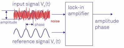
Figure 1. Lock-in amplifiers are capable of measuring the amplitude and the phase of a signal relative to a defined reference signal, even if the signal is entirely buried in noise.

Lock-In Amplifier Working Principle

Lock-in amplifiers use the knowledge about a signal's time dependance to extract it from a noisy background. A lock-in amplifier carries out a multiplication of its input with a reference signal - also sometimes known as down-mixing or heterodyne/homodyne detection - and then applies an adjustable low-pass filter to the result.

This approach is called demodulation or phase-sensitive detection and isolates the signal at the target frequency of interest from all other frequency components. The reference signal is generated by the lock-in amplifier itself or provided to the lock-in amplifier and the experiment by an external source.

The reference signal is typically a sine wave but could have other forms as well. Demodulation with a pure sine wave enables selective measurement at the fundamental frequency or any of its harmonics. Some instruments use a square wave ^[9] to capture all odd harmonics of the signal and, as a result, systematic measurement errors are potentially introduced.

Both the time and the frequency domain, first for mixing and then for the filtering process, are explored in order to understand lock-in detection.

Dual-Phase Demodulation

In a typical lock-in measurement, the device under test (DUT) is driven by a sinusoidal signal, as illustrated in Figure 2(a). The lock-in amplifier determines the amplitude R and phase Θ using the device response V_s(t) as well as the reference signal V_r(t). The so-called dual-phase demodulation circuit is used for this purpose, as shown in Figure 2(b).

The input signal is split and separately multiplied with the reference signal and a 90 phase-shifted copy of it. The outputs of the mixers are passed through configurable low-pass filters, resulting in the two outputs X and Y, known as the in-phase and quadrature component.

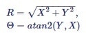
The amplitude R and the phase Θ are easily derived from X and Y by a transformation from Cartesian coordinates into polar coordinates using the following expression:

Equation (1)

 

It must be noted that atan2 is used instead of atan in order to have an output range for the phase angle that covers all four quadrants, i.e. (-Π, Π].

As shown in Figure 2(b), the lock-in amplifier has to split up the input signal in order to demodulate it with two different phases. Unlike analog instruments, digital technology overcomes any losses in SNR and mismatch between the channels when splitting the signal.

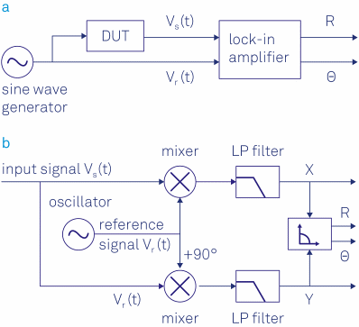
Figure 2. (a) Sketch of a typical lock-in measurement. A sinusoidal signal drives the DUT and serves as a reference signal. The response of the DUT is analyzed by the lock-in which outputs the amplitude and phase of the signal relative to the reference signal. (b) Schematic of the lock-in amplification: the input signal is multiplied by the reference signal and a 90° phase-shifted version of the reference signal. The mixer outputs are low-pass filtered to reject the noise and the 2ω component, and finally converted into polar coordinates.

Signal Mixing in the Time Domain

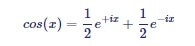
Complex numbers provide an elegant mathematical formalism to determine the demodulation process. The elementary trigonometric law is used for this purpose.

Equation (2)

 

to rewrite the input signal V_s(t) as the sum of two vectors in the complex plane, each one of length R/√2 rotating at the same speed ω_s, one clockwise and the other counter-clockwise:

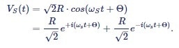Equation (3)

 

In the graphical representation given in Figure 3 (a) and (b), it can be observed that the vectors' sum projected on the x-axis – the real part – is exactly V_s(t), while the vector sum projection onto the y-axis – the imaginary part – is always zero.

The dual-phase down-mixing is mathematically expressed as a multiplication of the input signal with the complex reference signal:

Equation (4)

 

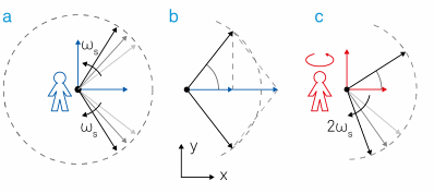
Figure 3. Demodulation process represented in the complex plane. (a) The input signal V_s(t) can be expressed as the sum of two counter-rotating vectors. (b) The projections onto the x-axis add up whereas the projections to the imaginary y-axis cancel each other out. (c) In the rotating frame the counter-clockwise vector is standing still, the clockwise moving vector rotates at twice the observer's angular velocity. Note that by convention, Θ is positive if the counter-clockwise vector is ahead of the reference.

The complex signal after mixing is expressed as follows:

Equation (5)

 

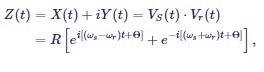
with signal components at the sum and the difference of the signal frequency and the reference frequency. The complex mixing is equivalent to an observer positioned at the origin and rotating in a counter-clockwise direction with frequency ω_r, as shown in Figure 3 (c).

In the eyes of this observer, the two arrows appear to rotate at different angular velocities ω_s - ω_r and ω_s + ω_r, with the arrow ω_s + ω_r rotating at a much faster rate if the signal and reference frequencies are close.

The subsequent filtering is mathematically expressed as an averaging of the moving vectors over time, indicated by the angle brackets <...>. Filtering removes the fast rotating term at |ω_s + ω_r| by setting {exp[- i(ω_s+ω_r)t+iΘ]}=0. Then, the averaged signal after demodulation becomes

Equation (6)

 

In the case of equal frequencies ω_s = ω_r, this expression is further simplified to

Equation (7)

 

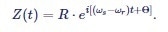
Equation 7 is the demodulated signal and the lock-in amplifier’s main output: with the absolute value |Z| = R given as the root-mean-square amplitude of the signal and its argument arg(Z) = Θ given by the phase of the input signal corresponding to the reference signal.

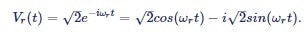
The real and imaginary components of the demodulated signal Z(t) are the in-phase component X and the quadrature component Y. They are derived using Euler's formula exp(iω_st) = cos(ω_st) + isin(ω_st) as:

Equation (8)

 

In the graphical view, ω_s = ω_r indicates that the arrow rotating counter-clockwise will appear at rest. The other arrow is rotating clockwise at double the frequency, i.e. -2ω_s, and is often called the 2ω component. Generally, the low-pass filter completely cancels out the 2ω component.

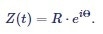
Figure 4 shows the various signals before and after mixing and filtering as they would appear on an oscilloscope. Figure 4(a) illustrates the sinusoidal example signals V_s and V_r over time that have exactly the same frequencies ω_s and ω_r.

The signal after mixing (blue trace in Figure 4 (b)) is dominated by the 2ω component. Only the DC component (green trace) remains following filtering and is equal to the in-phase amplitude X of V_s. If the signal frequency and the reference frequency deviate (Figure 4(c)), the resulting signal subsequent to mixing is no longer a simple sine wave and averages out to zero after filtering (Figure 4(d)).

It is the perfect example of synchronous detection, which exclusively extracts signals coherent with the reference frequency and discards all others.

Figure 4. (a) An input signal V_s (red) with peak amplitude of 0.5 V is multiplied with the reference signal V_r (blue) at the same frequency. (b) The resulting signal has a DC offset and a frequency component at twice the frequency of V_s and V_r. The DC value is 0.17 V, which is the in-phase component X of the input signal. (c) The input signal V_s is multiplied by a reference V_r at a different frequency. (d) The resulting signal has frequency components at f_s - f_r and f_s + fr. The average signal is always zero.

Signal Mixing in the Frequency Domain

The Fourier transform ^[10] is used to switch between the time domain and the frequency domain picture. It is linear and converts a sinusoidal function with frequency f₀ in the time domain into a Dirac delta function δ(f- f₀) in the frequency domain, i.e. a single peak at frequency f₀ in the spectrum.

As it is possible to express any periodic signal as a superposition of sines and cosines ^[11], transformations of signals comprising of only a few spectral components can often be intuitively understood.

Figure 5(a) displays a noisy sinusoidal represented in the time domain, which is then Fourier transformed into the frequency domain in Figure 5(b). The sinusoidal signal shows up as a peak both at +f_s and at -f_s in the spectrum. The smaller peak at zero frequency is due to the DC offset of the input signal.

The blue trace in Figure 5(c) represents the time domain signal after mixing. The associated spectrum (Figure 5(d)) is essentially a copy of the one in (b) shifted by the reference frequency f_r towards lower frequencies.

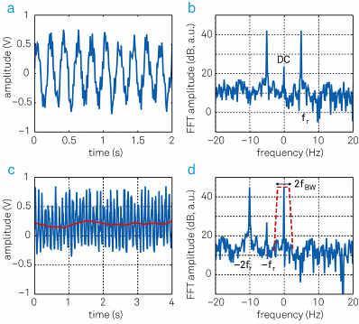
Figure 5. Relationship between time and frequency domain representation before and after demodulation. (a) Sinusoidal input signal superimposed with noise displayed over time. (b) Same signal as in (a) represented in the frequency domain. (c) After mixing with the reference signal (blue trace) and low-pass filtering (red trace), the signal spectrum up to f_BW remains. (d) In the frequency representation, the frequency-mixing shifts the frequency components by - f_r. The filter then picks out a narrow band of f_BW around zero. Note the component at frequency - f_s, which comes from offset and 1/f noise in the input signal. To obtain accurate measurements this component has to be suppressed by proper filtering.

Low-pass filtering is represented as a dashed red trace in (d) and chooses the frequencies up to a certain filter bandwidth f_BW. The output signal (red trace in (c)) is the DC component of the spectrum visualized in (d) and the noise contribution within the filter bandwidth |f| < f_BW.

These results clearly show that a filter bandwidth considerably smaller than the signal frequency f_s is required to efficiently suppress offsets in the input signal. Further criteria for choosing suitable filter characteristics in a given experimental situation are discussed in the following sections.

Low-Pass Filtering in the Frequency Domain

For the low-pass filtering, the frequency domain is considered first because there is a simple relationship between the incoming signal Q_in(ω) and the filtered signal Q_out(ω) for most filters as expressed below:

Qout(ω)=H(ω)Qin(ω).

Equation (9)

 

H(ω) is known as the transfer function of the filter. Q_in(ω) and Q_out(ω) are the Fourier transforms of the time domain input signal Q_in(t) and output signal Q_out(t), respectively.

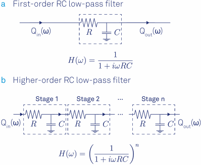
Figure 6. (a) First-order RC filter and its transfer function formula. (b) Steeper roll-offs towards higher frequencies are achieved by stacking multiple RC filters. The transfer function results from a multiplication of each filter's transfer function.

To perfectly reject unwanted components of the spectrum, it could be suggested that an ideal filter should have full transmission for all frequencies below f_BW, i.e. the passband, and zero transmission for all other frequencies, also called the stop band.

However, such idealized “brick-wall filters” are impossible to realize as their impulse response extends from -8 to +8 in time, making them non-causal.

As a basic approximation, the RC filter model is considered (Figure 6). It is easy to implement this type of filter in the analog and the digital domain. The transfer function of an analog RC filter is well approximated by:

Equation (10)

 

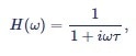
where t = RC is known as the filter time constant with the resistance R and capacitance C. The blue traces in Figure 7(a) and (b) illustrate this transfer function in Bode plots, 20log|H(2Πf)| and arg[H(2Πf)] as functions of log(f).

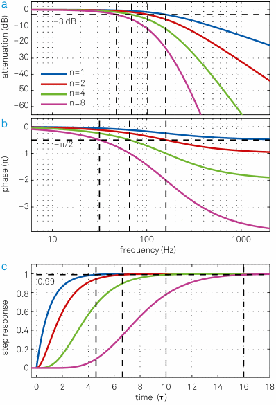
Figure 7. The blue traces in (a) and (b) show the transfer function H(ω) of an RC filter in the form of a Bode plot. The transfer functions for higher-order filters (n = 2, 4, 8) with the same filter time constant t are also plotted and clearly have much lower signal bandwidth f_-3dB. (c) Associated step response functions in the time domain. Cascading multiple filters leads to a significant increase in settling time to achieve the same level of accuracy. This is related to the larger phase delay that is inferred from (b). One additional nice feature of the cascaded RC or integrator filter is that it has no overshoot in the time domain, which is an issue with Butterworth filter for instance.

From the blue curve in Figure 7 (a) it can been seen that the attenuation grows 10 times every tenfold frequency increase above f_-3dB. This equals 6 dB/octave (20 dB/decade) corresponding to an amplitude reduction by a factor of 2 every doubling of the frequency. The cut-off frequency f_{- 3dB} is described as the frequency at which the signal power is lowered by -3dB or one half. The amplitude that is in proportion to the square root of the power, is decreased by1/√2 = 0.707 at f_-3dB.

For the filter expressed by Equation 10, the cut-off frequency is f_-3dB = 1/(2ΠT). Figure 7 (b) shows that the low- pass filter also introduces a frequency dependent phase delay equal to arg[H(ω)].

The first-order filter has a relatively poor roll-off behavior compared to the idealized brick-wall filter. Normally, many of these filters are cascaded in order to increase the roll-off steepness. The filter order is increased by 1 for every filter added. As the output of one filter becomes the input to the subsequent filter, their transfer functions can be simply multiplied. The following transfer function of an nth order filter is obtained from subsection 9:

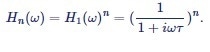Equation (11)

 

Its attenuation is n times the attenuation of a first-order filter, with a total roll-off of n x 20 dB/dec. Figure 7 (a) and (b) show the frequency responses of a 1^st, 2^nd, 4^th and an 8^th order RC filter. The higher the filter order, the closer the amplitude transfer function gets to a brick-wall filter behavior.

At the same time, the phase delay increases with filter order. For applications where the phase is used to apply a feedback to a system, for instance, phased-locked loops, any additional phase delay can limit the control loop’s stability and bandwidth.

The Bode plots for filters of various orders with the same bandwidths f_-3dB but different time constants are shown in Figure 8(a) and (b). The numerical relationship between corresponding filter properties is provided in Table 1.

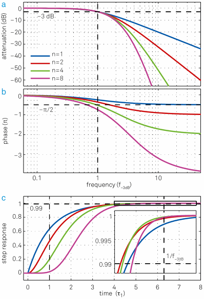
Figure 8. Same set of plots as for Figure 7 but this time all filters have the same cut-off point f_{- 3dB} but different time constants t = 0.16, 0.10, 0.069, 0.048. (a) Higher-order filters show a steeper roll-off towards higher frequencies. (b) Higher-order filters have larger phase delays, which can be detrimental for feedback applications. (c) Step response as a function of time in units of the time constant t 1 of the first-order filter. Though lower-order filters respond more quickly to changes of the input signal at the beginning, this advantage decreases over time and at some point higher-order filters even “overtake” lower-order filters, as seen in the inset.

Table 1. Overview of the filter properties of nth order RC filters with the same time constant. Dynamic applications usually take into consideration f_-3dB and settling times, whereas for noise measurements taking into account the correct f_NEP is key to achieve accurate results. With the relations given above one can easily calculate filter time constants for filters of the same bandwidth but different order.

Order n	Time constant T	Roll-off		Bandwidth in units of 1/T			Settling times in units of T
		dB/oct	dB/dec	f-3dB	fNEP	fNEP/f-3dB	63.2%	90%	99%	99.9%
1	1	6	20	0.159	0.250	1.57	1.00	2.30	4.61	6.91
2	1	12	40	0.102	0.125	1.23	2.15	3.89	6.64	9.23
3	1	18	60	0.081	0.094	1.16	3.26	5.32	8.41	11.23
4	1	24	80	0.069	0.078	1.13	4.35	6.68	10.05	13.06
5	1	30	100	0.061	0.069	1.12	5.43	7.99	11.60	14.79
6	1	36	120	0.056	0.062	1.11	6.51	9.27	13.11	16.45
7	1	42	140	0.051	0.057	1.11	7.58	10.53	14.57	18.06
8	1	48	160	0.048	0.053	1.10	8.64	11.77	16.00	19.62

 

For noise measurements, it is often more useful to specify a filter in terms of its noise equivalent power bandwidth f_NEP, instead of the 3 dB bandwidth f_-3dB. The noise equivalent power bandwidth is the cut of frequency of an ideal brick-wall that transmits the same amount of white noise as the filter to be specified. The conversion factor between f_NEP and f_-3dB is given for cascaded RC filters in Table 1.

Once the input signal V_s(t) is mixed with the reference signal √2 exp(-iω_rt), the input signal spectrum is shifted by the demodulation frequency ω_r and becomes V_s(ω- ω_r). Low-pass filtering further transforms the spectrum through a multiplication by the filter transfer function H_n (ω). The demodulated signal Z(t) contains all of the frequency components around the reference frequency, weighted by the filter response.

Equation (12)

 

Equation 12 clearly reveals that demodulation behaves like a bandpass filter, in that it selects the frequency spectrum centered at f_r and extending on each side by f_-3dB. It also shows that the spectrum of the input signal around the demodulation frequency f_r can be recovered by dividing the Fourier transform of the demodulated signal by the filter transfer function. FFT spectrum analyzers often use this form of spectral analysis, which is also called zoomFFT ^[12] .

Low-Pass Filter in the Time Domain

The time domain characteristics of a filter are best visualized by its step response (Figure 7(c) and Figure 8(c)). These plots correspond to a situation where the filter input is changed in a step-like fashion from 0 to 1. A certain amount of time will be required before the filter output settles at the new value.

The experimentalist must wait for a settling time long enough before performing the measurement in order to measure a signal that has passed through a filter accurately.

Table 1. lists the times to reach 63.2%, 90%, 99% and 99.9% of the final value for filters of different orders but identical time constant t. It is assumed that a 1 MHz signal is available and a 4th-order filter with a bandwidth of 1 kHz around 1 MHz is preferred to be used.

From the numbers listed in Table 1, it can be assumed that the settling time to 1% error is 0.7 ms and the time constant is 69 µs.

Signal Dynamics and Demodulation Bandwidth

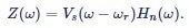
Setting the demodulation bandwidth is usually a tradeoff between time resolution and SNR. An amplitude modulated (AM) input signal with carrier frequency f_c = ωc/2Π is considered here.

Vs(t)=[1+hcos(ωmt)]cos(ωct+φc)

Equation (13)

 

Figure 9 illustrates how requirements for different experimental questions can be satisfied. The signal amplitude R(t) = 1 + hcos (ω_mt) (blue trace in Figure 9) is modulated at a frequency f_m= ω_m/2Π around the average value 1, where the modulation strength is characterized by the modulation index h. For this example, carrier and modulation frequencies of f_c = 2 kHz and f_m = 100 Hz, respectively, are selected.

Figure 9. Amplitude modulated signal: the green trace is the carrier input signal (displayed at a lower frequency for clarity). The blue trace indicates the signal amplitude, which is the envelope of the input signal.

Using the complex representation introduced with Figure 3, Figure 10(a) depicts the AM signal after mixing. Its angle φc is constant but its modulus |1 + hcos(ω_mt)| is time-dependent. The term cos(ω_mt) is the sum of the two counter-rotating vectors exp(iω_mt) and exp(-iω_mt).

These two vectors represent upper and lower sidebands of the frequency spectrum of an amplitude modulated signal, as shown in Figure 10(d). The quadrature and in-phase component are shown in Figure 10(b) and (c), respectively.

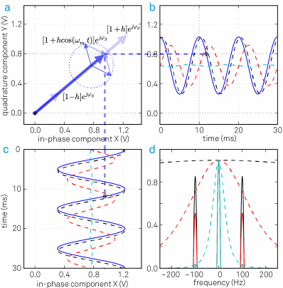
Figure 10. (a) An amplitude modulated signal in the rotating frame of reference is a vector with a time dependent length. The instantaneous signal is represented by the thick blue arrow; the thinner arrows display the two sidebands of the AM signal. (b) and (c) the quadrature and in-phase components of the demodulated input signal: the blue trace is the unfiltered signal, the dashed black, red and cyan traces are the filtered signals with f_-3dB = 500 Hz, 100 Hz and 20 Hz, respectively. (d) The frequency spectrum of the demodulated signal after filtering with three different bandwidths (black, red and cyan curves).

For most applications, one of the following quantities needs to be measured:

• the time dependence of the amplitude R(t) = 1 + hcos(ωmt)
• the average value of the amplitude {R(t)}
• the modulation index h

In the first situation, the demodulated signal is preferred to follow amplitude changes at a rate f_m. A filter bandwidth considerably larger than f_m is required for this purpose, for example, a 4^th-order filter with a bandwidth of f_{- 3dB} = 500 Hz.

With this choice, the transmission at f_m = 100 Hz (that is 100 Hz away from the carrier f_c) is about 98.5% and the phase delay is about 20° as can be calculated from Equation 11 and Table 1. In other words, the filter only has a slight effect on the modulation signal. The demodulated signal is shown as the dashed black line in Figure 10(b) and (c).

In addition to the desired sidband suppression/admission and phase delay, the amount of noise in the measurement is a critical criterion in the selection of a filter. Figure 11 illustrates this with an AM signal with relatively strong noise after demodulation in (a).

Panel (b) displays the same signal following filtering with a cutoff frequency equal to the modulation frequency. While this filter removes most of the noise, it introduces systematic changes in the phase and amplitude that must be corrected to obtain accurate results.

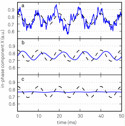
Figure 11. (a) A noisy input signal will produce a noisy demodulated signal, blue trace. The underlying signal without the noise is plotted as a black dashed trace. (b) Applying a filter with bandwidth f_-3dB = f_m = 100 Hz will eliminate most of the noise but will also affect the detected signal. (c) Same as (b) but with f_-3dB = f_m/5 = 20 Hz.

Frequency components corresponding to the sidebands are rejected by lowering the filter bandwidth to a value smaller than f_m for the second set of requirements. A 4th-order filter with f_-3dB = 20 Hz (dashed cyan line in Figure 10 (d)) suppresses the sidebands by 0.03 or 30 dB. The effect of such a strong filter on the measurement is illustrated in Figure 11(c).

The modulation index h needs to be known in the third case, but it is not required to resolve full signal dynamics. This is employed, for example, in Kelvin probe force microscopy, where h is a measure of the electrostatic force between a probe and a sample in response to an alternating voltage at f_m.

As the modulation index varies in proportion to the amplitude of the sidebands, it is possible to perform this measurement by applying narrow filters around the sidebands at f_c- f_m and f_c+f_m. Tandem demodulation and direct sideband demodulation are the two ways to do this.

In tandem demodulation, a wide-band demodulation is first performed around the center frequency. The resulting signal, which typically resembles the one in Figure 11(a), is then demodulated again at f_m. The modulation frequency accessible with this method cannot be greater than the maximum demodulation bandwidth of the first lock-in unit.

In direct sideband demodulation, the signal is demodulated at f_c ± f_m in one step, and the accessible modulation frequencies are only limited by the lock-in amplifier’s frequency range. Direct sideband demodulation also works with a single lock-in amplifier rather than two and is therefore usually the preferred option.

Achieving High SNR

In general, decreasing the filter bandwidth causes higher SNR at the expense of time resolution. What other measures can be carried out to improve SNR?

If it is not possible to increase the signal strength, the noise needs to be decreased or avoided as much as possible. However, noise always exists in analog signals and is caused by different sources, some of which are of fundamental origin, for instance, Johnson-Nyquist (thermal) noise, flicker noise, and shot noise, while others are of technical origin, for instance, interference, ground loops, 50–60 Hz noise, cross-talk or electromagnetic pick-up.

The magnitude of a random voltage noise Vnoise(t) is specified by its standard deviation. In the frequency domain, noise is characterized by its power spectral density |V_n(ω)|2 in units of V²/Hz, or by |V_n(ω)| in units of V/√Hz.

Figure 12 shows the qualitative spectrum, where different noise sources have different frequency dependencies. While Johnson-Nyquist noise has a flat spectrum for all practical frequencies and contributes to the “white noise”, flicker noise has 1/f frequency dependence (“pink noise”).

If there is some freedom in the choice of modulation frequency, a part of the spectrum where the noise level is lowest can be zoomed in to. Often higher frequencies where the spectrum comprises of white noise characteristics work best.

This approach is illustrated in Figure 12, where the amount of noise within the filter, as represented by the blue and gray filled area, is larger, for instance, in the lower frequency 1/f noise region. Therefore, the SNR at f₂ is higher than at f₁ using the same filter bandwidth, due to the fact that the noise density is low as long as other noise sources, such as wireless and radio transmission, are avoided.

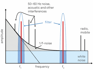
Figure 12. Qualitative noise spectrum of a typical experiment. The measurement frequency should be chosen in a region with small background, avoiding any discrete peaks coming from technical sources. In the example, f₂ will yield better results than f₂ for the same filter bandwidth, since it is located in a clean white noise region above the 1/f noise at low frequencies.

To provide a more quantitative example, let's assume a sinusoidal signal with amplitude of 1 µV across a 1 MΩ resistor with a SNR larger than 10 is to be measured. Such a resistor R exhibits a thermal noise with a power spectral density of , which amounts to about at T = 300 K room temperature¹. Here, thermal noise is found to be the dominant noise source and is clearly higher than the lock-in input noise of typically less than 10 nV/√Hz. The SNR can then be calculated as follows:

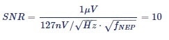Equation (14)

 

Equation 14 is solved for f_NEP to calculate that a NEP filter bandwidth of 620 mHz or less needs to be selected to achieve a SNR of 10. A 4th order filter is selected for this purpose. Using Table 1, the corresponding cutoff frequency f_-3dB = 549 mHz, the time constant t = 126 ms, and the settling time to 1% = 1.26 s, can all be calcuated.

As the noise amplitude is proportional to the square root of the bandwidth, the filter bandwidth needs to be decreased by a factor of 100 to further increase the SNR by a factor of 10. As a result, the settling time to 1% increases to over two minutes.

The lock-in technique is capable of supporting such long measurements as it is immune to DC offset drift in the input signal. However, other sources of drift such as changes in the amplifier gain, or in the DUT resistance, may influence long measurements. It is crucial to maintain stable conditions and especially constant temperature.

State of the Art

Lock-in amplifiers have come a long way since their invention in the early 1930s. Starting from vacuum tubes as basic instrument technology, the transformation to digital is well underway but not yet complete.

Digital lock-in amplifiers instantly convert the input signal to the digital domain with an analog-to-digital converter (ADC) and then perform all subsequent steps numerically with digital signal processing (DSP), as shown in Figure 13(b).

Conversely, in analog lock-in amplifiers, analog elements such as simple RC filters, voltage-controlled oscillators, and mixers are used for signal processing. Hybrid versions ^[9] are also available, as shown in Figure 13(a), which digitize the signals only after the analog mixing stage before or after filtering.

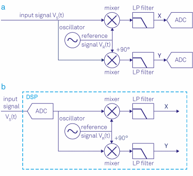
Figure 13. (a) Analog lock-in amplifier: the signal is split into two paths, mixed with the reference signal, filtered and then converted to digital. (b) Digital lock-in amplifier: the signal is digitized and then multiplied with the reference signal and filtered.

The transformation from analog to digital was driven by the availability of ADCs and DACs with ever increasing resolution, speed, and linearity. This development helped to push the input noise, dynamic reserve, and frequency range to new limits.

Also, digital signal processing is much less susceptible to errors introduced by a mismatch of signal pathways, to cross-talk and to drifts, caused, for example, by temperature changes. This is especially important at higher frequencies.

However, the biggest advantage of the digital approach is probably the ability to study the signal in multiple ways simultaneously with no loss of SNR.

As mentioned before, this allows not only better dual-phase demodulation, but also the investigation of several frequency components of a signal directly, without the need for cascading multiple instruments with all the accompanying detrimental effects.

After the transition from analog to digital, another key development is the availability of field programmable gate arrays (FPGA) with high computing power and abundant memory and speed. FPGAs are well known as digital clockworks that can be flexibly programmed to perform almost any desired signal processing task in real time.

The natural extension of the lock-in is to incorporate domain and frequency domain analysis before and after demodulation, which is something that would otherwise be carried out with a separate scope and spectrum analyzer. Also, a single instrument can consist of boxcar averagers to study signals with low duty cycle, PID and PLL controllers for feedback loops, and arithmetic units to process measurement data in real time.

The measurement signals can then be transmitted to a computer for further analysis. If an analog interface to another instrument is required, measurement data from different functional units is easily converted back to the analog domain using high-resolution DACs.

In 2013, Zurich Instruments introduced UHFLI ^[13], which is recognized as the most advanced instrument in terms of speed and level of integration. The front panel of UHFLI is shown in Figure 14. The instrument has a signal input bandwidth of 600 MHz and a maximum demodulation bandwidth of 5 MHz, making it the fastest commercially available lock-in amplifier.

Despite the high speed, UHFLI still delivers outstanding input noise performance of only 4 nV/√Hz and a dynamic reserve of 100 dB. Figure 16 shows the main functional components of the UHFLI and their interconnections, illustrating the high level of integration. Functionality that used to require an entire rack of instruments is now available in a single instrument no larger than a shoe box.

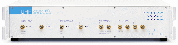
Figure 14. Zurich Instruments UHFLI Lock-in amplifier representing the state of the art of lock-in technology. The 600 MHz signal input bandwidth as well as the 5 MHz demodulation bandwidth make it by far the fastest lock-in amplifier on the market today. In addition, the 19 inch wide instrument integrates the greatest amount of functionality, see Figure 16, while providing the most advanced instrument control software LabOne^® (see Figure 15).

Clearly, it is not possible to control and utilize the wealth of functionality shown in Figure 16 with a few knobs and buttons on the front panel. Instead, the UHFLI is fully controlled from a computer running instrument control software called LabOne^®, which uses the latest browser technology, providing a graphical user interface to any device with a web browser (Figure 15).

High-level tools such as the PID Advisor, Parametric Sweeper, and the Software Trigger, utilize the available processing power of the host computer for measurement tasks, improving confidence in measurement results and enabling a more efficient workflow.

Additionally, LabOne^® also provides programming interfaces for MATLAB^®, LabVIEW^®, C#, and Python for seamless integration of the measurement instrument into existing experiment control environments.

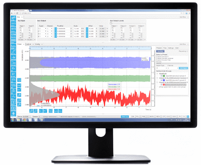
Figure 15. The LabOne^® user interface of the UHFLI Lock-in amplifier uses the latest web browser technology. The instrument can be controlled from multiple browser sessions on multiple PCs, tablets, etc. at the same time. Every signal analysis and control tool has a dedicated tab. Some of the functionality is intuitively displayed in form of block diagrams.

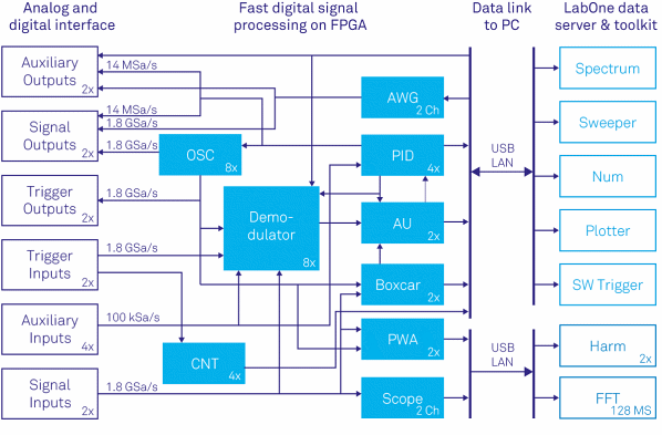
Figure 16. Block diagram showing the Zurich Instruments UHFLI's main functional entities and the signal flow between them. Fast digital signal processing takes place inside the instrument's FPGA clocked at 450 MHz but also on the computer connected by USB or 1GbE running the instrument control software LabOne^®. The main functional components inside the instrument are the 8 dual-phase demodulators, an oscilloscope (Scope) with digitizer functionality (DIG) and FFT , PID modules with PLL capability, an arithmetic unit (AU), a boxcar averager with periodic waveform analyzer (PWA) and a pulse counter module (CNT). For signal generation the instrument provides sinusoidal signal generators (OSC) and arbitrary waveform generators (AWG) for complex signal shapes. The LabOne control software running on the PC adds a parametric sweeper, a spectrum analyzer, a numerical parameter display (Num), a plotter, a software trigger for time domain analysis and a harmonic analyzer (Harm).

References

[1] C. R. Cosens. A balance-detector for alternating-current bridges. Proceedings of the Physical Society, 46:818, 1934.

[2] W. C. Michels. A Double Tube Vacuum Tube Voltmeter. Rev. Sci. Instrum., 9:10, 1938.

[3] W. C. Michels and N. L. Curtis. A Pentode LockIn Amplifier of High Frequency Selectivity. Rev. Sci. Instrum., 12:444, 1941.

[4] Interview of Robert Dicke by Martin Hawrit.Niels Bohr Library and Archives, College Park, MD: American Institute of Physics, www.aip.org/history-programs/niels-bohr-library/oral-histories/4572, 1985. Accessed: 2016-10-21.

[5] Zurich Instruments HF2LI. http://www.zhinst.com/products/hf2li. Accessed: 2016-10-21.

[6] A. M. Skellett. The Coronaviser, an Instrument for Observing the Solar Corona in Full Sunlight. Proc Natl Acad Sci USA, 26 (6):430, 1940.

[7] D. C. Tsui, H. L. Stormer, and A. C. Gossard. Two-dimensional magnetotransport in the extreme quantum limit. Phys. Rev. Lett., 48:1559, 1982.

[8] L. Gross et al. Bond-Order Discrimination by Atomic Force Microscopy. Science, 337(6100):1326, 2012.

[9] Stanford Research SR844. http://www.thinksrs.com/products/SR844.htm. Accessed: 2016-10-21.

[10] Wikipedia Article: Fourier Transform. https://en.wikipedia.org/wiki/Fourier_transform. Accessed: 2016-10-21.

[11] Wikipedia Article: Fourier Series. https://en.wikipedia.org/wiki/Fourier_series. Accessed: 2016-10-21.

[12] N. Thrane. Zoom-FFT. Brüel & Kjær Technical Review, (2):3, 1980.

[13] Zurich Instruments UHFLI. http://www.zhinst.com/products/uhfli. Accessed: 2016-10-21.

This information has been sourced, reviewed and adapted from materials provided by Zurich Instruments.

For more information on this source, please visit Zurich Instruments.