What is Optical Emission Spectrometry (OES) for Metal Analysis?
Thermo Scientific has been a longstanding provider of optical emission spectrometry (OES) solutions for metal analysis since 1934. Over this time, performance attributes such as accuracy, stability, and reliability have remained central to the development of its spectrochemical instrumentation.
Optical emission spectrometry is widely used in metals manufacturing for elemental composition analysis and quality control of solid metal samples.
The Thermo Scientific™ ARL iSpark™ 8860 Plus Metal Analyzer is a trusted standard that incorporates cutting-edge advancements to meet today's optical emission needs. It is designed to accurately and rapidly measure all elements of interest, meeting customers’ current and future needs for aluminum alloy sample analysis. The analyzer supports a wide range of metals analysis applications for incoming material control, process QC, final product QC, certification, or investigation.
The instrument is engineered for continuous operation and consistent analytical performance under recommended operating conditions.
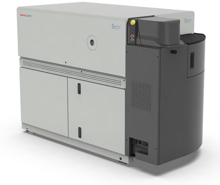
Image Credit: Thermo Fisher Scientific – Handheld Elemental & Radiation Detection
How Does Spark OES Work for Aluminum Alloys?
The Trusted Standard in Metal OES
The ARL iSpark 8860 Plus is based on a reliable one-meter focal-length vacuum-purged PMT spectrometer with a Paschen-Runge attachment.
This configuration supports high optical resolution and stability across a broad range of elements.
Key system features include:
- Advanced signal acquisition and processing to support analytical performance
- The Thermo Scientific™ intelliSource™, a digital spark source designed for flexible excitation conditions
- A redesigned spark stand to reduce maintenance and minimize memory effects
- ECO modes to reduce argon consumption during idle periods
- Integrated maintenance management tools to support system reliability
IntelliSource Digital Spark Source
The IntelliSource is a double current-controlled spark source that enables the development of optimized spark current profiles for:
- Sample surface preparation
- Material ablation
- Light emission across different metal matrices
Pre-integration spark conditioning supports improved sample homogenization, helping to reduce matrix and metallurgical effects prior to signal acquisition. Integration current profiles can be adjusted to support analysis of both trace elements and major alloying constituents.
Single Spark Acquisition (SSA) and Signal Processing
The analysis is performed by using high-frequency sequences of short-duration sparks. Each spark generates an individual emission signal, which is collected and digitized by photomultiplier tubes (PMTs).
Signal processing techniques include:
- DISIRE (DIffuse Spark Intensity REmoval) and FAST (Flexible Acquisition STart/Stop) to support signal quality.
- Spark-DAT algorithms evaluate non-metallic inclusions.
Time-Gated Acquisition (TGA)
TGA is an upgraded variant of TRS (Time-Resolved Spectroscopy). Signal capture occurs within specific TGA windows, short time intervals within individual flashes.
The start time and duration of the window are tuned for each analytical line to enhance the signal of interest while minimizing noise and the number of collected interferences. This supports improved detection limits, precision, and accuracy for multiple elements.
What Are Detection Limits and Precision in OES?
The ARL iSpark 8860 Plus metal analyzer provides defined performance in terms of detection limits (DL) and precision.
- Detection Limit (DL): The minimum concentration distinguishable from a blank with a defined probability, typically calculated as three times the standard deviation of the background signal.
- Limit of Quantification (LOQ): Approximately three times the DL, representing the lowest concentration that can be quantitatively determined.
Precision expresses the closeness of concentration values between individual runs of an analysis. Lower variability (better precision) reduces the number of runs required to achieve high confidence in the results.
Performance values depend on factors including calibration, sample preparation, and material homogeneity.
How Is Calibration Performed in OES Instruments?
Accuracy and Calibration Approach
Accuracy in OES represents the agreement between measured values and certified reference values. It depends on several factors, including:
- The quality and certification of reference materials
- Instrumental parameters (e.g., optical resolution, spark conditions, TGA settings)
- The calibration model used
Each ARL iSpark 8860 Plus spectrometer is factory-calibrated using certified reference materials (CRMs) and validated standards. Calibration curves are generated using multivariable regression (MVR) models to account for matrix effects and spectral interferences.
The Thermo Scientific™ OXSAS Analytical Software enables on-site calibration and adjustment using the same modeling approach. Measurement uncertainty and precision values can be displayed for each analysis.
Factory calibration provides a validated starting point; however, analytical performance remains dependent on application-specific calibration and operating conditions.
What Is Required for Accurate OES Sample Preparation?
Proper sample preparation is required for reliable OES analysis. For aluminum alloys, the sample surface is typically prepared using:
- A lathe
- A milling machine
Surface condition and material homogeneity can significantly influence analytical results.
How Fast Is OES Analysis for Aluminum Alloys?
The average analysis time for aluminum alloys is less than 23 seconds from start to result display. It is important to note that adding inclusion analysis to the elemental analysis method does not significantly increase total analysis time.
Image Credit: Thermo Fisher Scientific – Handheld Elemental & Radiation Detection
Table 1. ARL iSpark 8860 Plus - Detection limits and precision values for aluminum alloys. Source: Thermo Fisher Scientific – Handheld Elemental & Radiation Detection
| ELEMENT |
Ag |
As |
B |
Be |
Bi |
Ca |
Cd |
Ce |
Co |
Cr |
Cu |
Fe |
Ga |
Hg |
In |
La |
*Li |
| Typical DL [ppm] |
0.08 |
1.7 |
0.08 |
0.001 |
0.4 |
0.04 |
0.16 |
1.6 |
0.08 |
0.07 |
0.25 |
0.25 |
0.07 |
0.3 |
0.16 |
0.3 |
0.007 |
| Guaranteed DL [ppm] |
0.11 |
2.5 |
0.15 |
0.0012 |
0.6 |
0.1 |
0.3 |
2.3 |
0.12 |
0.15 |
0.4 |
0.6 |
0.1 |
0.4 |
0.3 |
1 |
0.02 |
| Level |
Precision (same unit as the concentration level) |
| 0.5 ppm |
|
|
0.05 |
0.01 |
|
|
|
|
|
|
|
|
|
|
|
|
|
| 1 ppm |
0.03 |
|
0.07 |
0.02 |
|
0.06 |
|
|
|
|
|
|
0.04 |
|
|
|
0.04 |
| 2 ppm |
0.04 |
|
0.1 |
0.04 |
|
0.08 |
0.08 |
|
0.04 |
0.06 |
0.2 |
|
0.07 |
0.2 |
|
|
0.07 |
| 5 ppm |
0.06 |
0.6 |
0.15 |
0.07 |
0.15 |
0.14 |
0.14 |
|
0.08 |
0.1 |
0.2 |
0.26 |
0.12 |
0.3 |
|
|
0.15 |
| 10 ppm |
0.1 |
0.8 |
0.2 |
0.1 |
0.25 |
0.2 |
0.22 |
0.5 |
0.13 |
0.2 |
0.3 |
0.4 |
0.21 |
0.4 |
|
|
0.25 |
| 20 ppm |
0.13 |
0.9 |
0.3 |
0.2 |
0.4 |
0.3 |
0.35 |
0.7 |
0.2 |
0.3 |
0.3 |
0.6 |
0.34 |
0.55 |
0.55 |
0.5 |
0.4 |
| 50 ppm |
0.22 |
1.1 |
0.6 |
0.5 |
0.7 |
0.5 |
0.7 |
1.1 |
0.4 |
0.6 |
0.5 |
1 |
0.67 |
0.8 |
0.9 |
0.8 |
0.9 |
| 100 ppm |
0.32 |
1.3 |
1 |
(1.7) |
1.5 |
0.8 |
1.6 |
1.6 |
1 |
1 |
1 |
1.5 |
1.1 |
1.5 |
1.3 |
1.2 |
1.5 |
| 200 ppm |
0.5 |
3 |
1.5 |
(3.6) |
3 |
1.3 |
3 |
2.3 |
2 |
1.5 |
2.1 |
2.5 |
1.8 |
2.7 |
2 |
2 |
2.5 |
| 500 ppm |
|
7 |
|
(9.4) |
6 |
2.6 |
6 |
3.7 |
5 |
4.5 |
4.7 |
7 |
3.6 |
|
|
3 |
5 |
| 1000 ppm |
|
|
|
|
11 |
|
|
|
10 |
8 |
8.6 |
12 |
|
|
|
|
|
| 0.2 % |
|
|
|
|
0.0018 |
|
|
|
0.002 |
0.0015 |
0.0016 |
0.0015 |
|
|
|
|
|
| 0.3 % |
|
|
|
|
|
|
|
|
0.003 |
0.002 |
0.0022 |
0.0025 |
|
|
|
|
|
| 0.5 % |
|
|
|
|
|
|
|
|
0.005 |
0.0035 |
0.0035 |
0.0045 |
|
|
|
|
|
| 1 % |
|
|
|
|
|
|
|
|
0.01 |
0.0065 |
0.0063 |
0.009 |
|
|
|
|
|
| 2 % |
|
|
|
|
|
|
|
|
|
|
0.012 |
0.016 |
|
|
|
|
|
| 3 % |
|
|
|
|
|
|
|
|
|
|
0.016 |
|
|
|
|
|
|
| 4 % |
|
|
|
|
|
|
|
|
|
|
0.021 |
|
|
|
|
|
|
| 5 % |
|
|
|
|
|
|
|
|
|
|
0.026 |
|
|
|
|
|
|
| 10 % |
|
|
|
|
|
|
|
|
|
|
0.047 |
|
|
|
|
|
|
| 20 % |
|
|
|
|
|
|
|
|
|
|
0.085 |
|
|
|
|
|
|
| ELEMENT |
Mg |
Mn |
Mo |
*Na |
Ni |
P |
Pb |
Sb |
Sc |
Si |
Sn |
Sr |
Ti |
V |
*Zn |
Zr |
| Typical DL [ppm] |
0.2 |
0.1 |
0.01 |
0.1 |
0.1 |
1.7 |
0.3 |
0.6 |
0.03 |
1 |
0.2 |
0.2 |
0.06 |
0.12 |
1 |
0.07 |
| Guaranteed DL [ppm] |
0.3 |
0.2 |
0.03 |
0.2 |
0.2 |
2.5 |
0.4 |
1 |
0.1 |
1.5 |
0.4 |
0.4 |
0.1 |
0.2 |
1.5 |
0.15 |
| Level |
Precision (same unit as the concentration level) |
| 1 ppm |
|
|
|
0.05 |
|
|
|
|
|
|
|
|
|
|
|
|
| 2 ppm |
0.1 |
0.07 |
0.08 |
0.08 |
0.06 |
|
0.1 |
|
|
|
|
|
0.15 |
0.1 |
|
|
| 5 ppm |
0.15 |
0.13 |
0.13 |
0.15 |
0.1 |
0.55 |
0.2 |
|
|
|
0.25 |
0.15 |
0.25 |
0.2 |
0.35 |
0.15 |
| 10 ppm |
0.2 |
0.2 |
0.2 |
0.25 |
0.2 |
0.7 |
0.3 |
0.4 |
0.4 |
0.5 |
0.35 |
0.2 |
0.35 |
0.25 |
0.51 |
0.2 |
| 20 ppm |
0.27 |
0.35 |
0.3 |
0.4 |
0.3 |
0.9 |
0.4 |
0.7 |
0.6 |
0.6 |
0.45 |
0.35 |
0.5 |
0.4 |
0.75 |
0.3 |
| 50 ppm |
0.4 |
0.6 |
0.55 |
0.8 |
0.6 |
1.3 |
0.7 |
1.3 |
2 |
0.9 |
0.7 |
0.6 |
0.75 |
0.7 |
1.2 |
0.5 |
| 100 ppm |
0.55 |
1 |
0.8 |
2 |
1 |
1.7 |
1.6 |
2.2 |
3 |
1.4 |
1 |
1 |
0.8 |
1.2 |
1.8 |
0.7 |
| 200 ppm |
1.5 |
1.6 |
|
4 |
2 |
2.2 |
3 |
3.5 |
4.5 |
2.5 |
1.5 |
2 |
1.8 |
2.3 |
2.7 |
1.1 |
| 500 ppm |
4.5 |
4 |
|
9 |
6 |
|
6.5 |
7 |
8 |
6 |
4 |
4 |
5 |
5 |
5 |
(3.5) |
| 1000 ppm |
8 |
7.5 |
|
|
10 |
|
11 |
13 |
12 |
10 |
8 |
6.5 |
11 |
9.5 |
8.5 |
(10) |
| 0.2 % |
0.0014 |
0.0014 |
|
|
0.002 |
|
0.002 |
0.003 |
0.002 |
0.0017 |
0.0017 |
0.0011 |
0.0024 |
0.0018 |
0.0014 |
(0.002) |
| 0.3 % |
0.002 |
0.002 |
|
|
0.0028 |
|
0.003 |
0.0043 |
|
0.0023 |
0.0025 |
|
0.0038 |
|
0.002 |
(0.003) |
| 0.5 % |
0.003 |
0.003 |
|
|
0.0044 |
|
0.0045 |
0.007 |
|
0.0034 |
0.0043 |
|
|
|
0.003 |
|
| 1 % |
0.0075 |
0.0057 |
|
|
0.009 |
|
0.008 |
0.014 |
|
0.0055 |
|
|
|
|
0.005 |
|
| 2 % |
0.015 |
0.011 |
|
|
0.041 |
|
0.014 |
|
|
0.009 |
|
|
|
|
0.0082 |
|
| 3 % |
0.023 |
|
|
|
0.066 |
|
|
|
|
0.014 |
|
|
|
|
0.011 |
|
| 4 % |
0.03 |
|
|
|
|
|
|
|
|
0.02 |
|
|
|
|
0.014 |
|
| 5 % |
0.035 |
|
|
|
|
|
|
|
|
0.025 |
|
|
|
|
0.017 |
|
| 10 % |
0.06 |
|
|
|
|
|
|
|
|
0.055 |
|
|
|
|
0.028 |
|
| 20 % |
0.11 |
|
|
|
|
|
|
|
|
0.1 |
|
|
|
|
|
|
| 30 % |
|
|
|
|
|
|
|
|
|
0.16 |
|
|
|
|
|
|
Comments on DL Values
- DLs and precision figures are based on at least six repeat measurements.
- The guaranteed DLs are determined with a 95 % confidence limit.
- Precision values are typical. The guaranteed precision values are 1.5 times higher, except for values in brackets, which are only typical due to element inhomogeneity at the relevant concentrations.
- Thermo Scientific’s standard calibrations provide guaranteed precision values for specific concentrations. Precision figures for concentrations not covered by the standard calibrations are provided solely for informative purposes.
- The values are applicable to an ARL iSpark 8860 Plus configured as recommended. The performance of multi-matrix instruments varies depending on the analytical lines and grating.
- These values relate to samples prepared using the suggested procedure and with homogeneous element distributions. Homogeneity is determined by the sample's metallurgical structure, which is impacted by its composition and production process.
Other factors that influence the liquid melt include the quality of the sampling and mechanical deformation caused by rolling. A measured precision exceeding the guaranteed precision indicates that the element is segregated or has an inhomogeneous distribution at the 95 % confidence level.
- The values were obtained using Ar 48 with a purity of at least 99.998 %.
- *Li and Na values are for lines installed in the first order of diffraction, not on the direct beam.
- *Mg: The usual DL is 0.02 ppm, with a guaranteed DL of 0.07 ppm if the most sensitive line used for pure and ultra-pure aluminum analysis is available.
- *The typical DL for Zn is 0.4 ppm, with a guaranteed DL of one ppm if the most sensitive line used for pure and ultra-pure aluminum analysis is present.
What Is Inclusion Analysis in Metal Spectrometry?
Ultra-Fast Inclusion Analysis Capabilities
The ARL iSpark 8860 Plus metal analyzer supports two approaches for qualifying non-metallic micro-inclusions in aluminum alloy samples. Data is acquired by processing individual spark signals using Spark-DAT (Spark Data Acquisition and Treatment) methods.
The inclusion analysis is typically performed alongside elemental analysis, but it can also be performed separately.
Standard Inclusion Analysis: This method qualitatively determines the quantity and size of most nonmetallic inclusions.
Inclusion Analysis with VUV Option: This option provides a method for qualitatively determining the quantity and size of most nonmetallic inclusions, including those containing carbon (C), nitrogen (N), oxygen (O), and chlorine (Cl). These particular elements require specific VUV optics and PMTs, which are included.
How Stable Is Spark OES Performance Over Time?
Stability and Memory Effects
Instrument stability is an important factor in routine analysis. Under normal operating conditions, mid-term stability is typically within three times the short-term precision at a given concentration.
The spark stand design minimizes memory effects (carryover between samples). However, when analyzing both pure aluminum and alloyed materials, the use of separate analytical setups (e.g., electrodes, tables) may be recommended.
Conclusion
The ARL iSpark 8860 Plus metal analyzer integrates advanced optical emission spectrometry technologies to support elemental and inclusion analysis of aluminum alloys.
Key capabilities include:
- Stable and reliable spectrometer design
- Support for low detection limits and repeatable measurements
- Flexible calibration approaches using MVR models
- Integrated inclusion analysis methods
- Efficient analysis workflows with short cycle times
When used with appropriate calibration, sample preparation, and operating procedures, the system supports consistent analytical performance across a range of metal analysis applications.

This information has been sourced, reviewed, and adapted from materials provided by Thermo Fisher Scientific – Handheld Elemental & Radiation Detection.
For more information on this source, please visit Thermo Fisher Scientific – Handheld Elemental & Radiation Detection.