The following article talks about a new machine condition measurement system which integrates particle count data and elemental analysis information in two closely interlinked measurement phases. This machine condition tool is part of a new portable product that also measures lubricant condition using IR and viscosity to complete the whole condition monitoring picture. The focus of this article is to define the new methodologies that apply to the machine condition aspect of the new tool. The article compares current analytical methods used to quantify wear conditions and contrasts them with the new methods and methodologies the device uses. In conclusion, this article presents case studies that use the device to illustrate how the measurements compare to other analytical methods in various machine condition monitoring applications.
Introduction
Particle count and elemental identification answers two of the most crucial questions in oil analysis: “How many?” and “Where is it coming from?” These two measurements are the most important in any machine condition monitoring application. Using existing technologies, the particle count is frequently a pre-screen for conducting root cause analysis using SEM/EDX, XRF and in certain cases ferrography. These methods have known to be time consuming, expensive and very labor intensive. Other repetitive elemental tests are employed but they are particle size sensitive towards the small fines, and they do not provide the ideal solution for detecting normal to abnormal wear transition.
Machine condition through oil analysis is normally monitored by quantifying the size, number and elemental composition of wear particles created at the extremities of lubricated machine parts. The quantity and size of these wear particles has a direct association to a benign versus an abnormal wear state (Figure 1).
It is crucial to understand that a benign wear state in one type of machine will be different compared to another. In these situations, the type of wear mechanism coupled with the contact area, speed, load and lubricant condition all govern the quantity and size of the regular benign wear. This makes limit and alarm settings hard compared to cleanliness control applications where the total contamination level must comply with a maximum threshold. This threshold is a fixed limit (frequently specified by the OEM) and it is frequently small enough to be easily quantified by light blocking laser particle counters. Particle count standards like NAS1638 and ISO 4406 were developed precisely for these applications.
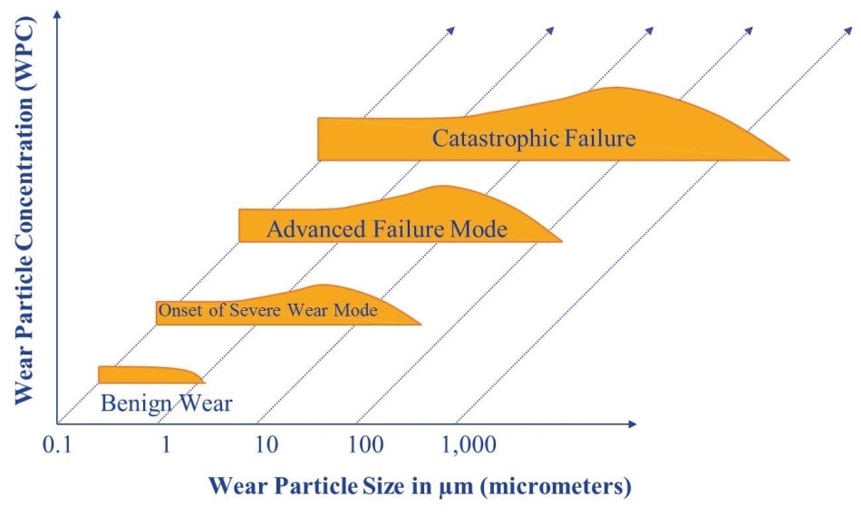
Figure 1. Progressions to Failure.
Filtration and other loss mechanisms in lubricant systems, which readily produce wear, also play a vital role in the whole particle picture. Filters are chiefly responsible for the condition of dynamic equilibrium for a specified particle size [1] and set baselines and alarms for large particles. Very fine particles do not function well in this model as they are diluted into the system, making any baseline measurement difficult. The transition from a usual benign wear mode to an abnormal wear mode also forms fewer small particles as the forces acting on the shear mixed layer are currently greater, and fine rubbing wear substitutes for a lot larger wear particles produced from underneath the shear mixed layer [2]. Machines create different types of wear particles based on the wear mode. These are explained in better detail in the Wear Particle Atlas [3].
Existing Machine Failure Measurement Techniques
Particle Count
Particle count is a good sign of the severity of a wear situation and the change from small to large particles can easily be detected. Particle count is typically performed using one of the following methods: direct imaging, laser light blockage or pore blockage.
Laser light blocking suffers from the ability to see through dark sooted samples and from coincidence effects (particle overlap). Thus, this process is restricted to clean translucent fluids used in the contamination control industry where internal machine contact is negligible.
Direct imaging counters the coincidence effect by processing particles over a larger area with the help of a CCD sensor. The sample illuminates by a pulsed laser diode which can increase light throughput and overcome dark sooted samples, to around 2% prior to dilution.
Traditional pore blockage devices are like optical particle counters as they saturate at comparatively low levels and are not perfectly suited to accurately quantify heavily contaminated machine wear samples. However, they have no trouble processing oils containing soot or water since these contaminants can travel through the pores without increasing the signal output. This is the main advantage that pore blockage methods have over light blocking and direct imaging methods.
LNF Compared to Traditional Ferrography
Atomic Emission Spectroscopy
Elemental identification of wear particles has traditionally been done using atomic emission spectroscopy by either Inductively Coupled Plasma (ICP) or Rotating Disc Electrode (RDE). Both these methods are inadequate in relation to identifying large particles. Thus, other complementary methods have been created to help increase the large particle detection capability of atomic emission. These methods include Rotrode Filter Spectroscopy (RFS) and acid digestion. These extra methods are time consuming and require plenty of special sample preparation and, in the case of acid digestion, hazardous chemicals are used.
X-ray Fluorescence (XRF)
XRF is a common method that quantifies separate chemical elements in used oil samples.
Samples are usually tested by taking an X-ray of a small oil sample (1-2 ml) in a cup. Similar to atomic emission methods, the large particles related with abnormal failure modes are not right for the analysis method using a cup as the focused XRF beam spot does not statistically signify the large particle distribution in just 1-2 ml of oil. These results do correlate well with RDE and ICP; however, the total elemental signal is a lot lower. Again, this is anticipated based on the small XRF beam spot compared to the total oil volume being studied. Interference from small sub-micron carbonaceous soot particles also creates problems for heavily sooted diesel engine oil samples using this method. These types of samples require some form of baseline calibration to compensate for the soot interference.
You can achieve better sensitivity for large wear particles by focusing the beam onto the particulate itself. This is fundamentally what happens when one analyzes particles from magnetic chip detectors using a piece of sticky tape. The RAF early failure detection centers (EFDCs) in the United Kingdom widely use this method.
Ferrography and Filter Patch Analysis
Microscopy is a robust method for identifying root causes of wear mode and mechanism failures. More advanced ferrography methods for substrate preparation also detect ferrous from non-ferrous metals and crystalline from non-crystalline materials. Ferrogram analysis is a thorough and conclusive test since it uses heat treatment to detect different types of steel together with particle color, morphology, surface and use of polarized light. The more advanced substrate preparation, such as using a ferrogram maker, varies from straight filter patch analysis in this respect.
The biggest disadvantage to performing ferrography is that it is time consuming and requires a highly skilled person to perform the analysis. This skill requires many years of testing multiple ferrograms to become skilled in the art. Microscopy methods need to be coupled with other quicker screening methods for them to be effective. It is not viable to run a repetitive sample history using just microscopy.

Figure 2. FPQ and XRF tower assembly.
SEM EDX
The SEM EDX method is used for visually analyzing particles at extremely high magnifications and performing spot elemental analysis on the particle with an EDX device. The depth of field is a lot larger on an SEM compared to conventional metallurgical microscopes. This depth of field improvement means the full particle can stay in focus at high magnifications and one can accomplish better detail.
Compared to standard wear particle analysis, using an optical microscope SEM EDX is not ideal for regular sample analysis. The instruments are expensive and the method requires some sample preparation, such as applying a conductive coating to the sample to help boost resolution of a full ferrographic analysis. However, if identification of the root cause of the issue is required or further corroboration is required, Spectro Scientific proposes a full Ferrography analysis.
A New Technique - Filtration Particle Quantification Combined with EDXRF
In this unique system design, machine failure and root cause analysis is inferred by using a two-step process integrating a modified pore blockage method with an XRF analyzer. Figure 2 illustrates the tower which encompasses the XRF and FPQ device in the total oil monitor system. The figure also illustrates the filter being inserted into the XRF. This comparatively fast process can screen out samples with high particle counts and perform a full 13 element XRF analysis on the resultant sample filter.
Combined Particle Quantifier (FPQ) and XRF Device
The adapted pore blockage method has been termed “Filtration Particle Quantification” (FPQ). The FPQ uses constant flow by driving a 3 ml oil sample using a syringe through a polycarbonate filter with ~30,000 4 µm diameter holes. The resultant pressure decline across the filter, measured with reference to atmospheric pressure is applied to quantify particles >4 µm up to ~1 million particles/ml. This is achieved primarily by using an altered filter design compared to a conventional pore blockage instrument. This new patent pending dual dynamic design allows a much greater particle count range (x50) beyond the point where particle swapping and saturation happens (refer Figure 3).

Figure 3. FPQ Filter vs Conventional Pore Blockage Filter.
Once the analysis is done, the filter moves from the FPQ to the XRF device. The FPQ and XRF are closely connected in terms of calibration because of the particle swapping occurrence. The FPQ and XRF instruments use a series of unique rules and calibrations to guarantee accurate elemental quantification of particles up to 1 million particles/ml. This method integrated with the patented filter overcomes the issue with the oil cup analysis which XRF devices normally use. This exclusive filter design can corral the particles into a small area on the filter so the focused X-ray beam can concentrate its energy on those particles. The instrument uses 40 keV and 15 keV to quantify 13 elements with an average limit of detection of ~1 ppm.
FPQ / XRF Device Case Studies
The case studies that follow show how the FPQ/XRF device correlates to current analytical methods for measuring particles in a variety of applications.
FPQ and X-Ray Correlation to Established Measurement Techniques
The following data set from a series of marine diesel vessels was used to assess the XRF and FPQ technology. Samples were tested on the FPQ device and XRF and were illustrated to correlate to LaserNet Fines® and acid digestion using the ICP. A model using an assumed wear particle size aspect ratio and particle mass was used to additionally correlate the aggregate elemental concentration on the FPQ filter using the LaserNet Fines® and XRF data. Figure 4 and Figure 5 illustrates how the FPQ and XRF correlate to the LaserNet Fines® direct imaging particle counter.

Figure 4. LaserNet Fines® vs. FPQ (counts/ml >4 µm).

Figure 5. LaserNet Fines® vs. XRF – Total ppm.
XRF vs. Acid Digestion
LaserNet Fines® direct imaging and spectroscopy are well proven methods to quantify particle count and elemental concentration, respectively. ICP and RDE spectrometers do not possess good sensitivity to detect large particles and they are used as trending tools for fine particles based on a dissolved elemental calibration. A recognized methodology to quantify large particles is to “acid digest” the whole sample by dissolving particles into a liquid which can be quantified using a typical ICP calibration. However, corrosive chemicals, cost, time, and effort make acid digestion impractical.
The data in Table 1 illustrates a range of marine samples tested on the ICP before and after acid digestion. This technique is typically known as differential acid digestion. Figure 6 illustrates how the differential ICP results (large particles) for samples E and F compare to the XRF data for the same samples. Note that the XRF data is not illustrated in Table 1. The large particle portion matches very well (within 3ppm) to the filtered XRF results (Figure 6).
Table 1. Differential Acid Digestion Sample Result (Sample E=10-1151, Sample F=10-1149).
| |
Before Acid Digestion - ICP (ppm) |
After Acid Digestion - ICP (ppm) |
| Sample |
A |
B |
C |
D |
E |
F |
A |
B |
C |
D |
E |
F |
| Ag |
0 |
0 |
0 |
0 |
0 |
0 |
0 |
0 |
0 |
0 |
0 |
0 |
| Al |
0 |
0 |
0 |
10 |
10 |
21 |
0 |
0 |
0 |
0 |
13 |
28 |
| Cr |
6 |
0 |
0 |
0 |
6 |
7 |
6 |
0 |
0 |
0 |
6 |
8 |
| Cu |
0 |
0 |
0 |
0 |
11 |
11 |
0 |
0 |
0 |
0 |
10 |
10 |
| Fe |
10 |
7 |
0 |
0 |
33 |
67 |
11 |
10 |
0 |
0 |
35 |
86 |
| Mo |
0 |
0 |
0 |
0 |
0 |
0 |
0 |
0 |
0 |
0 |
0 |
0 |
| Ni |
0 |
0 |
0 |
0 |
0 |
0 |
0 |
0 |
0 |
0 |
0 |
0 |
| Pb |
0 |
0 |
0 |
0 |
0 |
0 |
0 |
0 |
0 |
0 |
0 |
0 |
| Sn |
0 |
0 |
0 |
0 |
0 |
0 |
0 |
0 |
0 |
0 |
0 |
0 |
| Ti |
0 |
0 |
0 |
0 |
0 |
0 |
0 |
0 |
0 |
0 |
0 |
0 |
| V |
0 |
0 |
0 |
0 |
0 |
0 |
0 |
0 |
0 |
0 |
0 |
0 |
| Total ppm |
16 |
7 |
0 |
10 |
60 |
106 |
17 |
10 |
0 |
0 |
64 |
132 |

Figure 6. Differential ICP vs XRF (Sample E=10-1151, Sample F=10-1149).

Figure 7. Typical ratio of large to small particles observed between XRF and ICP (Sample F).
Figure 7 illustrates the difference in ppm between the ICP and XRF readings for Fe and Al in Sample F. This is an expected result based on how large and small particles act in a closed loop lubricating system. Large particles get lost and filtered out a lot more easily compared to fine debris which never gets lost and continues to increase in concentration.
PPM (Mass) vs Particle Concentration (Quantity) on the FPQ Filter
Based on the density of iron, it would take ~100 particles of the demonstrated dimensions in 1 ml of oil to raise the elemental concentration by only 1 ppm. For lighter metals such as aluminum, it takes about three times the amount of particles. This explains why the differential elemental ICP and XRF readings are comparatively low when compared to the fine and dissolved particle readings using regular spectroscopy. In this instance, the Fe and Al wear particles are most likely caused by cylinder/piston wear. This is a common failure mode in the application and reveals how the XRF can identify root causes of problems.

Wear Progression to Failure
When a machine enters an abnormal wear mode there is always a growth in the size and production of severe large wear particles. They are spotted as an increase from an established equilibrium level in the system. As the abnormal wear develops, the rate and size of production of these particles grows until the system ultimately fails. Note that fine wear particles detected by RDE spectroscopy and ICP continue to rise in the lube system and are not impacted by filtration or other system loss mechanisms.
Pay attention when changing the oil and then interpreting fine and dissolved wear metal data vs. XRF data. Limits based on rate of change apply in this situation. For larger particles measured by XRF and FPQ, a static limit applies after the system attains equilibrium. This is shown in Figure 8.

Figure 8. Behavior of large vs fine particles.
Unlike current optical particle counter and pore blockage technologies, the FPQ can handle a broad range of applications with comparatively high wear rates (up to 1.0 million p/ml). Table 2 illustrates FPQ and XRF data for a broad range of components that are usually found in heavy duty industrial vehicle equipment such as transmissions, final drives, engines and front differentials. The data reveals pairs of components with corresponding low and high wear rates.
Table 2. Normal and abnormal FPQ & XRF data for various applications.
| Sample |
Particle >4 µm (/ml) |
Application |
ITS Q5800 XRF (ppm) |
| LaserNet Fines |
FPQ data |
Al |
Cu |
Fe |
Si |
| E1 High Wear |
180209 |
141795 |
Engine |
2.0 |
0.0 |
0.8 |
1.4 |
| E2 Low Wear |
26802 |
44188 |
Engine |
0.5 |
0.6 |
0.6 |
0.7 |
| T1 High Wear |
46618 |
50390 |
Transmission |
0.4 |
2.2 |
2.2 |
1.7 |
| T2 Low Wear |
5346 |
9664 |
TransrnIsslon |
0.0 |
0.0 |
0.2 |
0.3 |
| F1 High Wear |
213674 |
226222 |
Final Drive |
4.3 |
0.0 |
8.4 |
7.0 |
| F2 Low Wear |
17185 |
26948 |
Final Drive |
0.1 |
0.0 |
2.0 |
0.5 |
| D1 High Wear |
88193 |
62259 |
Front Diff |
1.2 |
0.0 |
4.2 |
1.9 |
| D2 Low Wear |
37613 |
34773 |
Front Diff |
0.9 |
0.7 |
2.9 |
1.2 |
| E3 High Wear |
1025329 |
31686 |
Engine |
0.5 |
0.0 |
1.0 |
0.4 |

Figure 9. FPQ vs LaserNet Fines®, normal and abnormal wear in different applications.
As anticipated, the particle count on the FPQ correlates properly with direct imaging particle counting (Figure 9). Furthermore, the elemental XRF readings can distinguish between low wearing systems and more critical high wearing systems. This data illustrates that it is possible to make a proposal on the root cause of the increased wear rates based on a material map of the lube system.
This data set also shows a unique benefit that the FPQ has when testing emulsions and other sample types that have “phantom” particles included in the total particle count. Water and other liquids pass through the polycarbonate filter pores and the results are not influenced. Sample E3 contains a substantial amount of free water ingestion that produced a very elevated particle count reading on the LaserNet Fines®. The real particle count in this sample was just ~31 k p/ml and the elemental level was low.
Conclusion
The FPQ, with its patent pending dual dynamic filtration system, manages a broad range of lubricant applications with changing wear levels. The particle count using the FPQ filter correlates with current direct imaging particle counting. The following elemental concentration from the FPQ filter using XRF analysis connects well with ICP differential acid digestion, establishing that the methodology is successful. The combined particle count and elemental concentration recognizes varying wear rates and isolates potential root causes of issues in lube systems. Particle count and elemental concentration offers the real elemental break down of particles captured and quantified on the filter. This methodology removes many of the issues linked with other methods such as particle size detection and the resistant nature of many used oils found in heavy duty industrial applications.
References
[1] Daniel P. Anderson and Richard D. Driver. “Equilibrium particle concentration in engine oil” Wear, Volume 56, Issue 2, October 1979, Pages 415-419
[2] Reda, A.A., Bowen, E.R., and Westcott, V.C. “Characteristics of Particles Generated at the interface Between Sliding Steel Surfaces” Wear, Volume 34 (1975) Pages 261-273
[3] Anderson, D.P., “Wear Particle Atlas (Revised)” prepared for the Naval Air Engineering Center, Lakehurst, NJ 08733, 28th June 1982, Report NAEC-92-163, Approved for Public Release; Distribution Unlimited – Pages 125-134

This information has been sourced, reviewed and adapted from materials provided by AMETEK Spectro Scientific.
For more information on this source, please visit AMETEK Spectro Scientific.