Method for Increasing the SNR and Resolution of Images

Deconvolution is a computational technique of increasing the resolution and SNR (signal to noise ratio) of images captured on an imaging system. Its use existed before the extensive use of confocal microscopy, but due to the lack of computing power at the time, it was not commonly applied.

Today’s computing power, especially the massive parallelization of graphics processing units (GPUs), has broken down almost all barriers to entry, so that desktop PCs equipped with a suitable graphics card can implement deconvolution in almost real-time. This article introduces the concept of deconvolution as a day-to-day imaging tool that should be routinely applied to all images captured on a microscopy system.

Fusion, the latest microscopy imaging software from Andor, provides an optional deconvolution module called ClearView-GPU™. This enables the user to execute deconvolution and data acquisition simultaneously, providing rapid visualization of the original as well as deconvolved datasets on-screen and simplifying the user’s workflow. ClearView-GPU™ also includes a preview mode, which enables instant feedback of the effects of a range of deconvolution processing options and provides control over the result.

Key Features of Andor ClearView-GPU™

• Accurate – Accelerated Gibson-Lanni algorithm for accurate PSF estimates, supporting spherical aberration correction in deep specimens
• Powerful – GPU-accelerated enhanced Richardson-Lucy, Jansson-Van Cittert, and Inverse filtering algorithms
• Quantitative – “Energy conservation” matches total photon content of raw data and results
• Extremely fast – Optimized CUDA workflow for scorching performance
• Integrated – Combine with acquisition for “real-time” feeling or operate on stored data
• Sharper – better optical sectioning and enhanced contrast even in deep specimens
• Innovative – Richardson-Lucy iteration acceleration with gradient-driven convergence in fewer cycles

Image Formation

Image formation is the process through which an image of an object is projected by an optical system to a plane of observation or detection: the image is a spatial distribution of photons meant to represent the distribution of light emitted, reflected, or transmitted from an object of interest.

The “convolution” operation describes the image formation mathematically; in convolution, the spatial distribution of light collected from the object is convolved with the instrument point spread function (PSF). PSF is believed to be a fundamental property of the physical imaging system and sets a limit to spatial resolution. However, computer assisted imaging can cross this physical limit using methods such as deconvolution processing. The PSF shape is limited by diffraction, often at the pupil plane of the instrument.

As the PSF narrows, the spatial resolution increases and the (numerical) aperture of the optical system becomes larger. Convolution can be regarded as a mathematical description of blurring by the PSF, and it is this blurring which is sought to “undo”’ in deconvolution.

With regards to fluorescence microscopy, the SNR and the resolution limit the ability of a system to resolve an object. The following ways may affect the objects in the image:

• If the fluorescence intensity of an object is too close to the background intensity of the sample or noise floor of the detection system, it will not be visible
• If two objects are separated by less than the resolving power of the system, they will appear as a single object
• If an object is smaller than the system’s resolving power, it will appear at least as large as the resolution limit of the system

In the following sections, the deconvolution is described mathematically and then visually in order to support a more intuitive understanding. The Fourier Transform (FT) is an important mathematical relationship relied upon in deconvolution. The FT is a way of describing distributions (commonly temporal or spatial), by a set or collection of alternative functions.

In order to convert to the FT, the phase and amplitude of a set of spatial frequencies which describe the original function is calculated. The outcome is a set of pairs of sines and cosines at different spatial frequencies, each pair with an amplitude or constant of intensity.

Calculation of this significant function has been improved over many generations and now with the use of GPU power, it can be calculated very quickly. It proves to be the case that when distributions are expressed by their FT, the convolution of spatial distributions is represented by multiplication, whereas deconvolution is represented by division. That simplifies computations quite a lot.

However, this simple relationship is applicable only for the ideal noise-free case. For real imaging situations, noise makes this more difficult and then iterative techniques have to be used.

Here, the simple case is illustrated in which the image received by the detector can be considered to be formed from a collection of points of light, each of which has been convolved with the PSF. As a visual example, the following test pattern of objects can be considered (Figure 1).

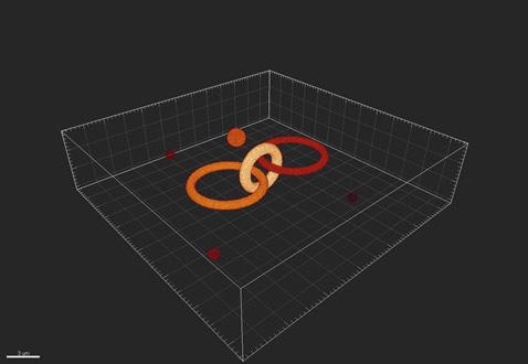
Figure 1. An example of the true objects being imaged by the imaging system.

Once the light has passed through the optics of the system and been received by the detector, it has been convolved or blurred so that the objects appear as represented in Figure 2.

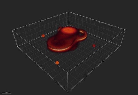
Figure 2. An example of how the imaging system might distort, or convolve, the objects.

Figures 3 and 4 show the blurring function or point spread function, which shows a 3D view and 2D projection, respectively. The rings in Figure 4 are called Airy rings, and are characteristic of an imaging system with a circular aperture.

Here, 70% of the transmitted energy is enclosed in the central bright spot and the extent of this spot is called one Airy unit, corresponding to 1.22*wavelength/NA, where wavelength is the emitted wavelength and NA the limiting aperture of the optical imaging system.

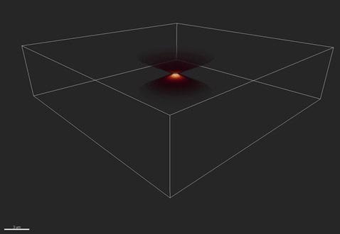
Figure 3. The distortion of a single point, or Point Spread Function (PSF). Shown here in 3D.

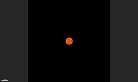
Figure 4. The PSF in 2D shows a series of rings - known as the “Airy pattern” - with an “Airy disk” at its center.

Since it is already known the way the image is convolved with the PSF as it passes through the imaging system, the inverse of this process to deconvolve the image and recover both signal and resolution can be applied.

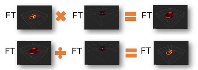
Figure 5. Simplified explanation of image convolution and its inverse, deconvolution to recreate the original object. Note that FT represents the Fourier Transform, which allows us, in the noise-free case, to replace convolution with multiplication and deconvolution by division. Thus at top, we see the image formation process, in simplified form and below the image recover or deconvolution process.

Nyquist Sampling

In the early 20^th Century, during the advent of digital electronics, Harry Nyquist (and various others) realized that in order to accurately represent a continuous (or analog) series in a discrete (or digital) way, the recording, or representation, of the continuous series should be at least twice its frequency.

The recording of audio into digital formats at a frequency of at least 40 kHz (typically 44.1 kHz or greater is used) is an everyday example of this phenomenon. This is due to the fact that the human auditory system (an analog recording device) is usually not capable of detecting frequencies above 20 kHz. In case the audio was recorded below 40 kHz, the high frequency treble sounds would be either lost or worse, aliased into lower, spurious frequencies.

The lower the recording frequency, the worse it would sound. This can be represented as follows:

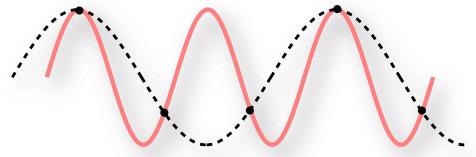
Figure 6. Under sampling a continuous signal.

The red line represents the continuous series which is to be recorded as a digital signal. The black dots are the frequency at which they are recorded. Therefore, the dashed line is the digital representation of the signal. It is clearly different from the original series!

A visual example of this case is the moiré pattern observed in images that are captured or resized at low resolution:

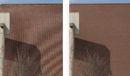
Figure 7. The image on the left has not been captured at sufficient resolution and shows artifacts.

In the case of imaging in three dimensions on a fluorescence microscope, the image size (or more technically, the pixel size) and the step size (Z) need to be set appropriately.

The limit of lateral (XY) resolution can be determined by the well-known Abbe equation:

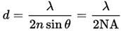
For instance, using 525 nm light and a high NA objective, such as a 1.4 oil, this is 188 nm.

Nyquist sampling theorem shows that the digital sampling should be at least twice this frequency (or half the distance), or that the pixel size (in the image plane) should not be greater than 94 nm. If a total magnification (C-mount and objective) of 100x is used, this equates to a 9.4 µm pixel on the camera.

The following formula reveals the limit of axial (Z) resolution:

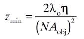
Where η is the refractive index of the medium.

Using the same example as before and 1.518 as the refractive index, this is 813 nm.

Nyquist sampling theorem shows that the Z-step size should therefore be no larger than 0.4 µm, or 406.5 nm.

Note: The more information that can be provided to the deconvolution processing, the better the resolution and SNR in the final image.

The smallest pixel size and the smallest Z-step practical should be used within the usual limitations of imaging with samples that may be sensitive to bleaching and/or phototoxicity.

The Fusion software from Andor includes options for increasing the sampling for Z-stacks in the Protocol Preferences and also provides users the option for increasing the magnification lens(es) of the Dragonfly system:

Figure 8. Strict Nyquist option in Fusion software.

Figure 9. Using the 2x lens on a Dragonfly system.

ClearView-GPU™: Fusion’s Deconvolution Module

The Image Processing section contains the Andor’s ClearView-GPU™ module.

If a CUDA-compatible GPU and driver is found, the GPU compatibility icon will show green and deconvolution processing will be up to 50 times faster than the processing done on the CPU. Both options are supported in the Fusion software.

Additionally, it includes options for previewing a region of the image for instant feedback of the results, enabling the user to adjust the processing settings and view their effects prior to applying them to an entire dataset.

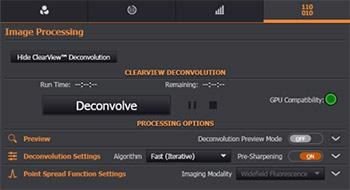
Figure 10. Fusion's Deconvolution module in the Image Processing Tab.

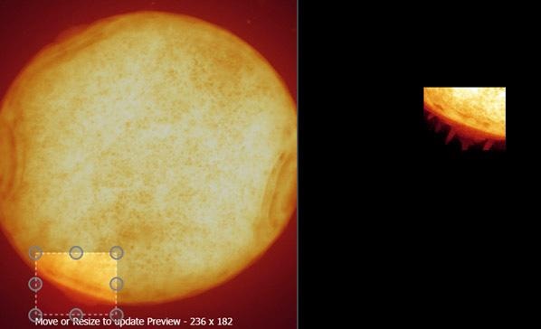
Figure 11. Preview allows a small region to be deconvolved instantly.

Algorithms and Point Spread Functions

There are three processing algorithms involved in ClearView-GPU™: Robust, Fast, and Fastest. Each represents a balance between image quality and processing time.

• Robust is an iterative maximum likelihood estimator, giving the best results and is also resistant to noise in the image
• Fast is also an iterative method and uses the Van Cittert method to lower the processing time, typically by a factor of two when compared to Robust.
• Fastest is non-iterative and uses an inverse (Wiener) filter to further reduce the processing time, again usually by a factor of two in comparison with Fast

In all cases, the dataset is divided into chunks for processing on the GPU (defined by the GPU Processing Memory Limit setting in the Rendering menu of the Preferences area in Fusion). This implies that there is no limit on the size of datasets that can be deconvolved; however, more GPU memory leads to faster processing times.

ClearView-GPU™ includes five PSF models. All the models use a fast integrator to speed up the Gibson-Lanni algorithm, used to estimate a robust 3D PSF, with aberrations. This is the best algorithm currently available for PSF estimation.

• Widefield Fluorescence
• Spinning Disk Confocal
• Brightfield
• TIRF
• Laser Scanning Confocal

Advanced Settings

The default settings have been chosen carefully to ensure that the best results are provided for most images. If users wish to adjust these settings, they can do so in the Deconvolution Settings section. It is suggested to do these settings whilst in Preview Mode to get an instant update of the effect of the setting.

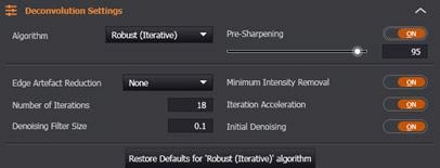
Figure 12. Fusion's Deconvolution module in the Image Processing Tab.

Although it is beyond the scope of this article to provide a comprehensive explanation of all of them, Minimum Intensity Removal is relevant in that users should disable this setting if they wish to maintain “energy conservation” and make sure that the photon (pixel) counts in their original and processed datasets are identical (< 1% discrepancy).

Results

Table 1. Comparison of imaging performance with the Dragonfly in widefield and confocal with 40 μm pinhole before and after deconvolution. Measurements were made with MetroloJ imageJ plugin for PSF analysis. 100 nm beads fluorescent were imaged at 488 nm laser excitation, with a Zyla 4.2 plus, 1X camera zoom and Nikon 60X/1.4 plan apo oil lens, Z step was 0.1 μm. FWHM is the full width at half maximum intensity across a line profile, a standard measure of the resolution.

PSF measurements	WF	WF + decon	DFly 40	DFly 40 + decon
Lateral FWHM (nm)	245	185	238	139
Lateral (XY) Projection
.	.	.	.	.
Axial (Z) Projection

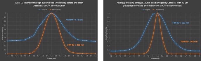
Figure 13. Axial through-series (normalized) intensity profile of 100 nm bead showing the increase in SNR and decrease in FWHM (increase in resolution) after deconvolution in both widefield and confocal.

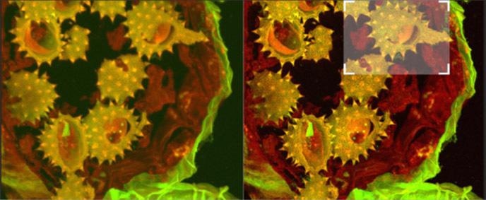
Figure 14a. Shows full field image of the daisy pollen grains before and after deconvolution, with merged channels viewed as a maximum intensity projection image. Note the contrast and detail enhancement in the deconvolved images. Because this is a bright robust specimen, we could extend exposure times to 250 ms, achieving high SNR to recover high spatial frequencies for deconvolution. Thus, we could exceed the Abbe diffraction limit in confocal imaging. But the density of the specimen is also a challenge to optical sectioning, as evidenced in the haziness of the single optical section in C. Daisy pollen maximum intensity projection of 488 and 561 channels before and after deconvolution with Fusion, imaged on Dragonfly with 488 and 561 laser excitation. A Zyla 4.2 PLUS was used with 1X camera zoom and Leica 100X/1.44 oil lens. Highlighted region shown below.

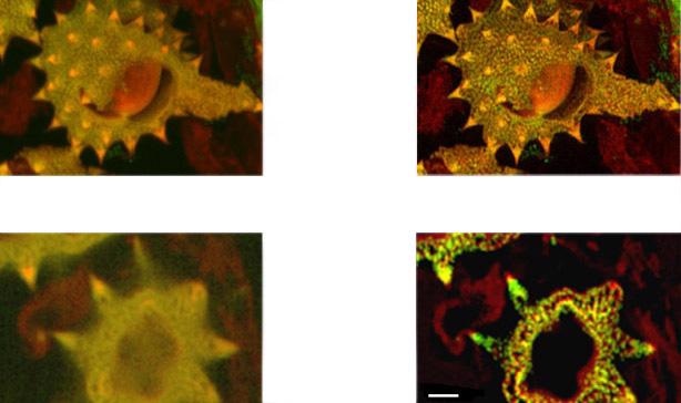
Figure 14b. (above). Shows detail at full resolution from image in A above. Surface clarity is enhanced as well as sharpness and resolution improvement in individual pollen grain. Fig 14 c (below) shows single optical section from two channel daisy pollen Z series. ClearView-GPU enhances contrast, sharpens optical sectioning and provides clear channel separation in this thick bright specimen. Fine structures within the walls of the pollen grains become clearly visible. These punctate features are in the range 150-200 nm FWHM after deconvolution. Scale bar is 2 μm.

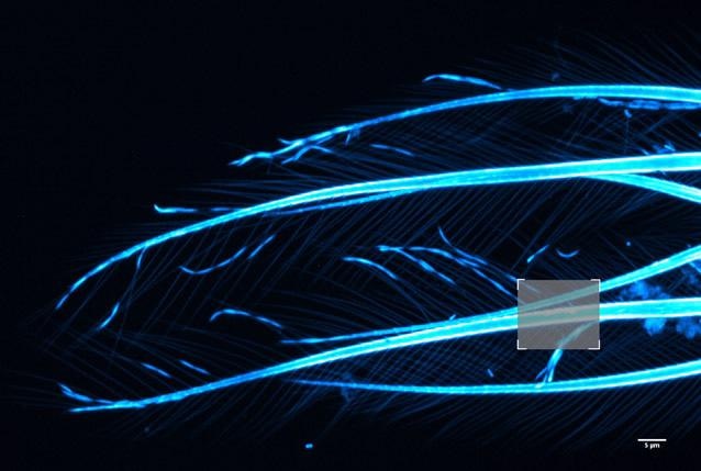
Figure 15. Brine shrimp tail captured with a 40 µm pinhole on Dragonfly. Objective is 63x1.4. Camera is Zyla 4.2 Plus sCMOS with additional 1.5x magnification lens in Dragonfly. Highlighted region shown over in Fig. 16 before and after ClearView-GPU™ deconvolution

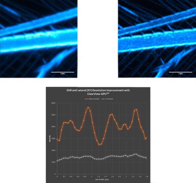
Figure 16. Confocal (top left); deconvolved (top right) and line profile (bottom) showing increase in SNR and lateral resolution. Notice the haze along the line profile in the confocal image becomes clearly separated as four distinct objects after deconvolution.

Speed Comparison

Andor ClearView-GPU™ has been designed to guarantee the highest speeds and functionality with the largest possible datasets.

Using identical hardware and as similar settings as possible, ClearView-GPU™ has been proven to be up to 10x faster than other leading GPU-accelerated packages and up to 50x faster than CPU-based methods, particularly for larger datasets, even when iteration acceleration is disabled.

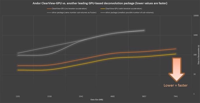
Figure 17. Confocal (top left); deconvolved (top right) and line profile (bottom) showing increase in SNR and lateral resolution. Notice the haze along the line profile in the confocal image becomes clearly separated as four distinct objects after deconvolution.

Application Example

In addition to the obvious visual benefit of deconvolution as described above, a more powerful advantage is how it can enhance the ability to accurately analyze images using the extensive collection of tools available to researchers.

The most spatially conserved data (highest contrast and clearest boundaries) to the target elements are required for investigation to achieve the most accurate analysis, be it a simple point-to-point measurement, or the more advanced auto-detection of a subcellular structure and potentially tracking it over time.

The vesicle tracking (Figure 18, below) is a good working example, for instance in autophagy models for cancer research. The size of vesicles lies in the range of a micron or less, and can be smaller than the pure resolution of an optical system without deconvolution. Moreover, they can be densely populated and also move fast in a three-dimensional volume.

Deconvolution can greatly enhance the ability to discreetly detect individual vesicles and allow dedicated software analysis modules (for example Imaris LineageTracker) to autodetect and analyze them for parameters such as direction, number, and distance traveled and speed of movement (Figure 19).

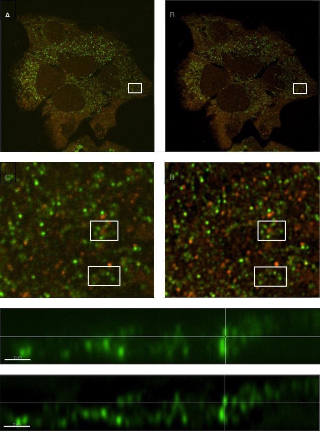
Figure 18. Comparison of a sample with labeled vesicles imaged using Dragonfly confocal mode (A, C & E) and following ClearView-GPUTM deconvolution (B, D & F). C and D show zoomed regions of A and B respectively, and within those regions, clusters of vesicles are much clearer to see in the deconvolved image (D) compared to the raw confocal image (C). E and F are orthogonal (x,z) views demonstrating smaller diameter profiles with higher contrast in the deconvolved image (F) owing to the reassignment of light omitted from each vesicle back to its origin.

Discussion

This article has shown how the use of ClearView-GPU™ deconvolution increases the resolution in all three dimensions, exceeding the Abbe limit in some cases. It also increases the SNR for all imaging modalities. Features that were not previously distinguishable become clearly separated.

Considering the power of modern GPUs and the storage space available on latest workstations, Andor’s ClearView-GPU™ deconvolution can be applied to every dataset from an imaging system.

Using Andor’s ClearView-GPU™ and Fusion software, deconvolution can occur in parallel with image acquisition or as a post-processing step, if required.

The original data is not altered as the deconvolved data is produced in addition to, rather than replacing, and can be applied in quantitative studies if energy conservation is ensured using the advanced settings.

Sources and Further Reading

• Castleman, 1979; Agard and Sedat, 1983; Agard et al., 1989
• Image by Pluke - Own work, CC0, https://commons.wikimedia.org/w/index.php?curid=18423591
• CC BY-SA 3.0, https://commons.wikimedia.org/w/index.php?curid=644816
• James Pawley “Handbook of Biological Confocal Microscopy” 3rd Edition, Chapter 1, Springer, 2006
• S. F. Gibson, F. Lanni, “Experimental test of an analytical model of aberration in an oil-immersion objective lens used in three-dimensional light microscopy,“ J Opt Soc Am [A] 1991 Oct;8(10):1601-13.
• P.A. Jansson “Deconvolution of Images and Spectra”, 2nd edition, Dover Publications, Academic Press, 1997, ISBN-13: 978-0-486-45325-5

This information has been sourced, reviewed and adapted from materials provided by Andor Technology Ltd.

For more information on this source, please visit Andor Technology Ltd.