Volatile organic compounds (VOCs) are chemicals that easily volatilize at low temperatures from certain solids and liquids.1 VOCs, for instance, xylene, can be released as organic chemicals from a wide range of sources.
VOCs see routine use in a diverse array of everyday products such as fuels, paints, and household cleaners, but they are known to lead to both short- and long-term health effects, from nose, throat, and eye irritation to lasting damage to the liver, kidneys, and central nervous system.2
The versatile gas chromatography-mass spectrometry (GC-MS)-based EPA Method 8260 can be used to determine VOC content in a range of sample matrices, including soil and water.
This method has been used to determine many VOCs, providing guidance on sampling techniques, sample preparation, and analysis. EPA Method 8260, referencing guidance from EPA Method 5021, states that it is possible to use headspace for the introduction of VOCs from water samples into a GCMS system.3
Headspace is a sample preparation technique suitable for the extraction of VOCs from liquid and solid matrices without the need for complex sample preparation.
This article validates a VOC analysis method for water samples using guidance from EPA method 8260. A combination of the SCION Instruments HT3 Headspace Sampler, the SCION 8300 GC, and the SQ 8700 MS is used in this work.
The HT3 Headspace Sampler can be used in static mode using a loop method. This instrument can also be converted into dynamic mode via a trap method. Results for VOC analysis in water using the HT3 in static mode are presented alongside analysis in dynamic mode to draw a comparison.
Experimental
An internal standard (IS) was implemented to improve the precision of the results, with fluorobenzene added at the same concentration to all samples. A working standard was also prepared at a concentration of 10 µg/mL in methanol.
Table 1. Instrument parameters for GC-MS. Source: SCION Instruments UK Ltd
| GC Part |
Settings |
| Injector (SSL) |
200 °C
Split 20:1 |
| Liner |
Narrow bore straight through |
| Column |
SCION 624-MS
30 m x 0.25 mm x 1.4 μm |
| Carrier Gas |
Helium
1.5 mL/minutes |
| Oven Program |
40 °C, hold five minutes
8 °C/minute to 180 °C, hold 0.17 minutes
30 °C/minute to 250 °C |
| Run Time |
25 minutes |
| Software |
MSWS |
| MS Part |
Settings |
| MS transfer line temp. |
230 °C |
| Ion source temp. |
250 °C |
| MS mode Electron |
Ionization |
| Delay collection time |
5 minutes |
| Scan mode |
SIM |
Commercially available VOC standards containing a range of VOC compounds were purchased. These compounds had a concentration of 2000 µg/mL (Table 4). It is important to note that not all compounds have been mentioned in the results section due to the number of compounds present in the standard.
A stock standard was prepared with a concentration of 1 µg/mL in water. This standard was then used to prepare linearity samples at five different concentration levels: 1, 5, 10, 30, and 100 ppb in water.
Each linearity sample included 100 ppb of IS. A total of 1 mL of each solution was added to individual headspace vials prior to analysis.
Water samples were prepared with 100 ppb of IS. QC-spiked water samples were prepared with 100 ppb of IS and spiked with 30 ppb of the VOC standard. One mL of sample was added to individual headspace vials for analysis, and 1 mL of water was added to headspace vials for solvent blanks.
Table 2. HT3 static headspace (Loop) settings. Source: SCION Instruments UK Ltd
| Variable |
Value |
| Constant Heat Time |
ON |
| GC Cycle Time |
35 minutes |
| Valve Oven Temp. |
120 °C |
| Transfer Line Temp. |
120 °C |
| Standby Flow Rate |
30 mL/minutes |
| Platen/ Sample Temp. |
70 °C |
| Platen Temp Equil. Time |
1 minute |
| Sample Equil. Time |
1 minute |
| Mixer |
ON |
| Mixing Level |
Level 5 |
| Mixing Time |
10 minutes |
| Mixer Stabilize Time |
0.5 minutes |
| Pressurize |
5 PSIG |
| Pressurize Time |
0.15 minutes |
| Pressure Equil. Time |
0.20 minutes |
| Loop Fill Pressure |
3 PSIG |
| Loop Fill Time |
1 minute |
| Inject Time |
0.50 minutes |
| Software |
HT3 TekLink |
Table 3. HT3 dynamic headspace (trap) settings. Source: SCION Instruments UK Ltd
| Variable |
Value |
| Trap |
Trap K Vocarb 3000 |
| Valve Oven Temp. |
140 °C |
| Transfer Line Temp. |
140 °C |
| Standby Flow Rate |
30 mL/minute |
| Trap Standby Temp. |
30 °C |
| Trap Sweep Temp. |
30 °C |
| Platen/ Sample Temp. |
70 °C |
| Sample Preheat Time |
0 minutes |
| Preheat Mixer |
ON |
| Preheat Mixing Level |
Level 5 |
| Preheat Mixing Time |
10 minutes |
| Preheat Mixer Stabilize Time |
0.50 minutes |
| Sweep Flow Rate |
40 mL/minute |
| Sweep Flow Time |
3 minutes |
| Dry Purge Time |
0.50 minutes |
| Dry Purge Flow |
50 mL/min |
| Dry Purge Temp. |
30 °C |
| Desorb Preheat |
270 °C |
| Desorb Temp. |
275 °C |
| Desorb Time |
5 minutes |
| Trap Bake Temp. |
300 °C |
| Trap Bake Time |
5 minutes |
| Trap Bake Flow |
50 mL/minute |
| Software |
HT3 Teklink |
Table 1 shows the instrument parameters for the GC-MS, while Tables 2 and 3 feature headspace sampler parameters for the HT3 in static mode (loop) and dynamic mode (trap), respectively.
The system demonstrated excellent specificity, and it was noted that compounds resolved well from one another while also exhibiting good peak shape.
Selective ion monitoring (SIM) was employed to enhance system sensitivity. A single quantifier ion and two qualifier ions were chosen for each VOC (Table 4).
The most abundant ion for each VOC was selected to be the quantifier ion. Qualifier ions underpin analyte confirmation, preventing the false identification of compounds. The second and third most abundant ions for each compound were chosen as qualifier ions.
Figure 1 features an example of the MSWS MS software, highlighting the selected quantifier and qualifier ions for 4-isopropyltoluene.
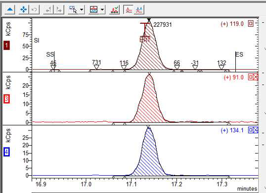
Figure 1. Example mass spectra of 4-Isopropyltoluene from linearity sample (30 ppb) ran using dynamic headspace sampling showing quantifier (top) and qualifier plots (middle and bottom). Image Credit: SCION Instruments UK Ltd
Results
The correlation coefficient (r2) and RSD for the system precision (n=6) for the selected VOCs using static headspace are shown in Table 4.
EPA Method 8260 states that the initial calibration should achieve r2≥0.99.3 The r2 values using static headspace were all found to be >0.996, with most >0.998, confirming excellent linearity.
Table 5 shows the r2 and RSD for system precision (n=5) of the selected VOCs using dynamic headspace. It was observed that r2 values obtained using dynamic headspace were all >0.98, with most >0.993.
EPA Method 8260 also notes that, because this method can be used to analyze a large number of compounds, some compounds are expected not to meet the acceptance criteria. As a result, the method allows 10% of compounds to exceed this r2 value.
EPA Method 8260 also states that calibration models may use an alternate fit, for example, forcing through the origin when appropriate for the current project, but it is deemed inappropriate to make changes to pass the QC criteria once the calibration has been finalized.
In the experiment presented here, it was determined that 29.2% of compounds analyzed had r2 values <0.99 when using dynamic headspace.
The method states that, where appropriate, data for compounds that fail to meet the criteria but are not vital to the specific project can be used as estimated values or qualified data for screening purposes.3
Figures 2 and 3 show calibration curves for 4-isopropyltoluene under static and dynamic headspace conditions, respectively.
Table 4. Correlation coefficient and system precision results for VOCs using static headspace. Source: SCION Instruments UK Ltd
| VOC |
Correlation
coefficient (r2) |
RSD (%) |
SIM Ions (Quantifier
and qualifiers) |
| 2-Chlorotoluene |
0.9988 |
2.98 |
91, 89,126 |
| 4-Isopropyltoluene |
0.9982 |
5.20 |
119, 91, 134 |
| Benzene |
0.9985 |
0.83 |
78, 77, 51 |
| 1,3,5-trimethylbenzene |
0.9986 |
5.29 |
105, 120, 77 |
| tert-Butylbenzene |
0.9984 |
4.07 |
119, 91, 134 |
| Ethylbenzene |
0.9982 |
2.82 |
91, 106, 65 |
| Isopropylbenzene |
0.9987 |
3.72 |
105, 120, 79 |
| m-Xylene & p-Xylene |
0.9983 |
2.96 |
91, 106, 105 |
| n-Propylbenzene |
0.9987 |
3.81 |
91, 120, 65 |
| o-Xylene |
0.9982 |
2.35 |
91, 106, 105 |
| sec-Butylbenzene |
0.9990 |
4.89 |
105, 134, 91 |
Table 5. Correlation coefficient and system precision results for VOCs using dynamic headspace. Source: SCION Instruments UK Ltd
| VOC |
Correlation
coefficient (r2) |
RSD (%) |
SIM Ions (Quantifier
and qualifiers) |
| 2-Chlorotoluene |
0.9953 |
9.14 |
91, 89,126 |
| 4-Isopropyltoluene |
0.9966 |
10.06 |
119, 91, 134 |
| Benzene |
0.9984 |
17.39 |
78, 77, 51 |
| 1,3,5-trimethylbenzene |
0.9963 |
9.55 |
105, 120, 77 |
| tert-Butylbenzene |
0.9964 |
10.04 |
119, 91, 134 |
| Ethylbenzene |
0.9972 |
9.20 |
91, 106, 65 |
| Isopropylbenzene |
0.9963 |
8.56 |
105, 120, 79 |
| m-Xylene & p-Xylene |
0.9967 |
7.39 |
91, 106, 105 |
| n-Propylbenzene |
0.9965 |
8.46 |
91, 120, 65 |
| o-Xylene |
0.9957 |
8.07 |
91, 106, 105 |
| sec-Butylbenzene |
0.9961 |
9.89 |
105, 134, 91 |
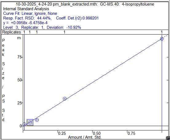
Figure 2. Example from linearity ran using static headspace sampling for 4- Isopropyltoluene, showing correlation coefficient (r2) from data review in MSWS. Image Credit: SCION Instruments UK Ltd
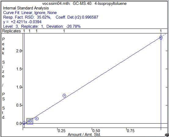
Figure 3. Example from linearity ran using dynamic headspace sampling for 4-Isopropyltoluene, showing correlation coefficient (r2) from data review in MSWS. Image Credit: SCION Instruments UK Ltd
Table 6. Recovery and precision results from spiked sample using static headspace. Source: SCION Instruments UK Ltd
| VOC |
Recovery (%) |
RSD (%) |
| 2-Chlorotoluene |
99.25 |
2.92 |
| 4-Isopropyltoluene |
91.86 |
4.74 |
| Benzene |
108.06 |
0.96 |
| 1,3,5-trimethylbenzene |
94.20 |
4.97 |
| tert-Butylbenzene |
95.33 |
3.73 |
| Ethylbenzene |
101.45 |
2.67 |
| Isopropylbenzene |
98.39 |
3.52 |
| m-Xylene & p-Xylene |
104.58 |
2.98 |
| n-Propylbenzene |
96.23 |
3.97 |
| o-Xylene |
101.84 |
2.57 |
| sec-Butylbenzene |
93.37 |
5.50 |
Table 7. Recovery and precision results from spiked sample using dynamic headspace. Source: SCION Instruments UK Ltd
| VOC |
Recovery (%) |
RSD (%) |
| 2-Chlorotoluene |
74.97 |
9.10 |
| 4-Isopropyltoluene |
70.79 |
10.04 |
| Benzene |
124.26 |
17.44 |
| 1,3,5-trimethylbenzene |
71.04 |
9.53 |
| tert-Butylbenzene |
70.17 |
9.99 |
| Ethylbenzene |
74.14 |
9.22 |
| Isopropylbenzene |
70.50 |
8.53 |
| m-Xylene & p-Xylene |
74.79 |
7.42 |
| n-Propylbenzene |
72.89 |
8.43 |
| o-Xylene |
69.34 |
8.11 |
| sec-Butylbenzene |
72.35 |
9.89 |
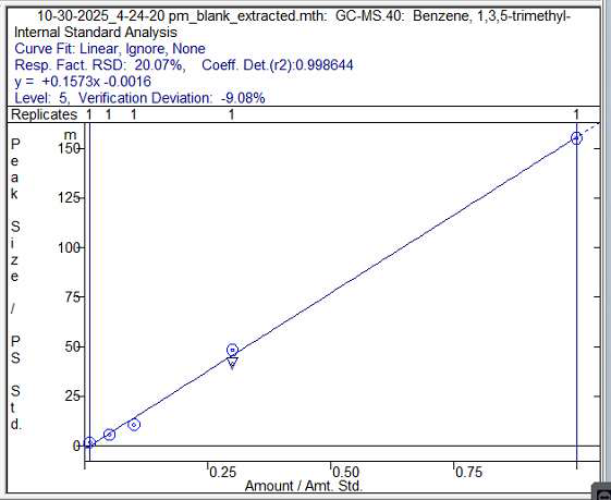
Figure 4. Example QC spiked sample ran using static headspace sampling for 1,3,5-trimethylbenzene from data review in MSWS, showing recovery of 90.92%. Image Credit: SCION Instruments UK Ltd
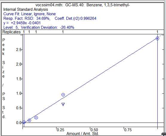
Figure 5. Example QC spiked sample ran using dynamic headspace sampling for 1,3,5-trimethylbenzene from data review in MSWS, showing recovery of 73.60%. Image Credit: SCION Instruments UK Ltd
For each target analyte using static headspace, the system precision was ≤6.8%. The RSD of VOCs analyzed using dynamic headspace was ≤12.8%.
EPA Method 8260 states that the RSD must be ≤20% for each target analyte. This was achieved using both static and dynamic headspace.
Precision and recovery results for QC-spiked samples of selected compounds, sampled using the static headspace (n=6), are shown in Table 6. Precision was found to be ≤5.5% and recovery was from 87.79–108.06% across all analyzed VOCs.
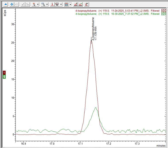
Figure 6. Example expanded TIC overlaid linearity sample (1 ppb) ran using dynamic headspace (red) and linearity sample (1 ppb) (green) ran using static headspace sampling for 4-Isopropyltoluene. Image Credit: SCION Instruments UK Ltd
Precision and recovery results for selected compounds’ QC spiked samples sampled using the dynamic headspace (n=5) are shown in Table 7. Precision was ≤17.44% across all VOCs analyzed, with most <11%.
Recovery was determined to be between 69.34% and 124.26%, but virtually every analyte achieved recovery in the 70–80% range.
The precision results for the QC spiked samples had an RSD ≤20% using static or dynamic headspace, meeting the criteria specified in the method.
The suggested acceptance criteria for the recovery of the target analytes in EPA Method 8260 are 70–130%.3 It was observed that QC-spiked samples sampled utilizing static headspace are comfortably within this range, while those sampled using dynamic headspace sit slightly outside these criteria on the lower end. For example, o-Xylene features a recovery of 69.34%.
Spiking the sample enables evaluation of the analytical method’s performance to ensure it delivers valid and accurate results. Spiking a sample increases target analyte concentration by a known amount, meaning it is possible to confirm that added analytes are recovered.
It is important to spike a sample at a concentration within the linearity range, without increasing sample volume. This ensures consistent calculations while avoiding the introduction of unknown effects.
Table 8. Signal comparison between static and dynamic headspace at 1 ppb. Source: SCION Instruments UK Ltd
| VOC |
Signal Dynamic
(KCps) |
Signal Static
(KCps) |
Ratio Dynamic
to Static |
| 2-Chlorotoluene |
17228.25 |
5330.09 |
3.12 |
| 4-Isopropyltoluene |
25632.66 |
6600.69 |
3.88 |
| Benzene |
8205.87 |
4923.46 |
1.67 |
| 1,3,5-trimethylbenzene |
29412.80 |
6526.78 |
4.51 |
| tert-Butylbenzene |
12469.76 |
2289.09 |
5.45 |
| Ethylbenzene |
24291.15 |
6370.08 |
3.81 |
| Isopropylbenzene |
16124.56 |
4106.94 |
3.93 |
| m-Xylene & p-Xylene |
58587.88 |
7865.19 |
7.45 |
| n-Propylbenzene |
21945.28 |
3948.41 |
5.56 |
| o-Xylene |
1996.31 |
7039.99 |
2.84 |
| sec-Butylbenzene |
14787.04 |
2634.52 |
5.61 |
Table 9. Signal to Noise comparison between static and dynamic headspace @1 ppb. Source: SCION Instruments UK Ltd
| VOC |
S/N Dynamic
(KCps) |
S/N Static
(KCps) |
Ratio Dynamic
to Static |
| 2-Chlorotoluene |
257.04 |
23.98 |
10.72 |
| 4-Isopropyltoluene |
2221.78 |
65.06 |
34.15 |
| Benzene |
108.56 |
28.32 |
3.83 |
| 1,3,5-trimethylbenzene |
721.43 |
50.27 |
14.35 |
| tert-Butylbenzene |
1088.02 |
37.10 |
29.33 |
| Ethylbenzene |
522.56 |
24.04 |
21.73 |
| Isopropylbenzene |
856.78 |
58.66 |
14.61 |
| m-Xylene & p-Xylene |
1143.36 |
39.54 |
28.92 |
| n-Propylbenzene |
323.17 |
14.09 |
22.94 |
| o-Xylene |
478.04 |
32.23 |
14.83 |
| sec-Butylbenzene |
451.93 |
16.54 |
27.32 |
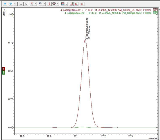
Figure 7. Example overlaid QC spiked sample (red) and water sample (green) ran using dynamic headspace sampling for 4-Isopropyltoluene. Image Credit: SCION Instruments UK Ltd
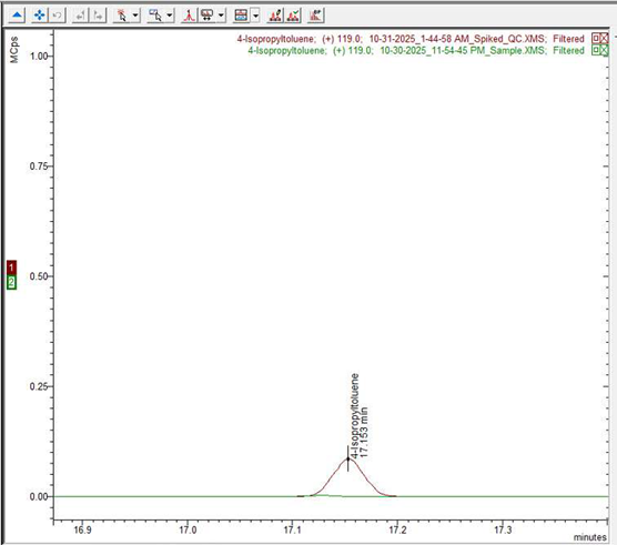
Figure 8. Example overlaid QC spiked sample (red) and water sample (green) ran using static headspace sampling for 4-Isopropyltoluene. Image Credit: SCION Instruments UK Ltd
Figures 4 and 5 feature an example data review in MSWS for 1,3,5-trimethylbenzene in a QC-spiked sample. This was analyzed using static and dynamic headspace. The verification deviation was used to calculate recovery before an average was calculated across the samples analyzed.
Figure 6 features an example of a sample containing 1 ppb 4-Isopropyltoluene. This was sampled using dynamic headspace (red) and static headspace (green) overlaid in the image. It can be seen that the 4-Isopropyltoluene peak that was sampled using dynamic headspace is considerably larger.
Table 8 highlights the signal differences between static and dynamic sampling for the selected compounds. The dynamic sampling results featured a larger signal than the static results. The ratio of dynamic to static results was found to range from 1.67 to 7.78 times greater signal.
Table 9 shows the signal-to-noise comparison between static and dynamic sampling for the selected compounds. The ratio of dynamic to static results was found to be 7.87–58.06 times greater in this instance.
Figures 7 and 8 feature examples of an overlaid QC-spiked sample and a water sample for 4-isopropyltoluene, analyzed using dynamic and static headspace, respectively.
These figures confirm that the signal for the QC-spiked sample is far greater when employing dynamic headspace. No VOCs were identified to be ≥LOQ using both static and dynamic headspace sampling.
Conclusion
This article validated a method for VOC analysis in water samples, drawing on EPA Method 8260 and employing the SCION Instruments HT3 headspace sampler in combination with the SCION 8300 GC and SQ 8700 MS.
The HT3 headspace sampler was used in static mode with a loop method and in dynamic mode with a trap method. Both sampling methods were found to achieve the LOQ of 1 ppb.
The study leveraged QC-spiked samples and an internal standard to verify a robust working method and to account for sampling variation, respectively.
It was possible to achieve good linearity, system precision, and recovery results with the majority of compounds meeting the acceptance criteria stipulated in EPA Method 8260. These criteria were met when using both static and dynamic headspace sampling, while analyzed water samples were confirmed to include no VOCs≥LOQ.
Using dynamic headspace sampling, larger signal and a higher signal-to-noise ratio were achieved than with static headspace sampling.
It is advisable to check with local regulatory authorities to ensure that all testing and reporting requirements are adhered to. The SCION applications team can also offer assistance.
References and Further Reading
- United States Environmental Protection Agency (2023). What are SVOCs (and VOCs)?. US EPA. Available at: https://www.epa.gov/east-palestine-oh-train-derailment/what-are-svocs-and-vocs.
- United States Environmental Protection Agency (2014). Volatile Organic Compounds” Impact on Indoor Air Quality. US EPA. Available at: https://www.epa.gov/indoor-air-quality-iaq/volatile-organic-compounds-impact-indoor-air-quality#Health_Effects.
- United States Environmental Protection Agency (2019). EPA Method 8260D (SW-846): Volatile Organic Compounds by Gas Chromatography-Mass Spectrometry (GC/MS). US EPA. Available at: https://www.epa.gov/esam/epa-method-8260d-sw-846-volatile-organic-compounds-gas-chromatography-mass-spectrometry-gcms.

This information has been sourced, reviewed, and adapted from materials provided by SCION Instruments UK Ltd.
For more information on this source, please visit SCION Instruments UK Ltd.