The particles within a powder sample are present in a wide variety of sizes, shapes and compositions; with the requirements on their analysis and characterization being just as diverse.
Analysis of particles could only need shape measurement from one field of view, or it could need a combination of shape and chemical measurement from thousands of particles over a large sample area.
Combining a table top microscope (TTM) with the AZtecFeature X-Ray Energy Dispersive Spectroscopy (EDS) system provides researchers a highly flexible platform for any type of particle analysis.
AZtecFeature uses the TTM to capture images which can then be used to find particles within a sample. The X-ray EDS detector captures a spectrum from each particle in the sample and, using the TTM’s motorized stage, this can be achieved over a large sample area – either for the analysis of widely distributed particles or to increase the sample population size.
The analyzed particles can be categorized according to their shape or their chemistry; either during the measurement or afterwards. These categorizations allow particles to be identified or to determine if further analysis must take place to ensure an accurate identification. Once analysis targets are reached the analysis can then be terminated.
Metal Powders – Determining Particle Size Characteristics and Contamination Levels
A titanium-based power was distributed over a carbon adhesive tab on a sample mount and placed in the TTM. The goal of the analysis was to determine the shape and size of the particles present and establish the identity of any possible contaminants.
AZtecFeature determines the location of particles in an electron image by the application of grey level thresholds. Setting the grey level thresholds in AZtecFeature is an interactive process, allowing the adjustment and tuning of the grey level threshold ranges to achieve the optimum detection of particles in the sample images.
In this instance one grey level threshold was applied to the backscattered electron (BSE) image to determine the location of particles and their shapes. A single field of view BSE image, which was used to adjust the grey level threshold, is shown on the left-hand side of Figure 1. The right-hand side of the image shows the impact of the grey level threshold and the particles detected by AZtecFeature.
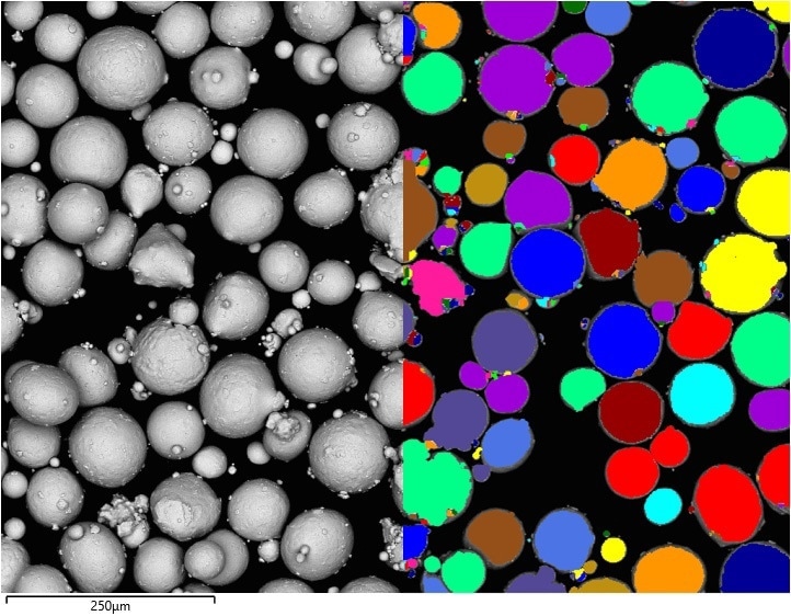
Figure 1. Left - Backscattered electron image of particles. Right - Grey level thresholding, colouring each particle that has been located – note that adjacent particles have clearly been separated. Image Credit: Oxford Instruments
As the images are captured the system determines the shape data for each particle (Figure 2) and an X-ray spectrum is taken to determine the particle’s chemistry. The automated nature of the TTM stage means that data can be collected over multiple fields of view, meaning the entire sample can be analyzed. For this sample a total area of 2.67 mm x 2.63 mm was analyzed over 12 separate images, with 328,235 particles detected.
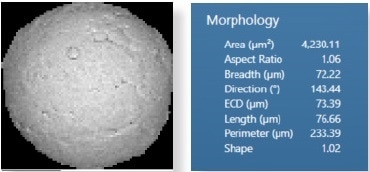
Figure 2. (A) Thresholded image of a particle from which its morphological parameters are measured. (B) Morphological values for the particle in Fig. 2A. Image Credit: Oxford Instruments
To create an appropriate categorization method for the sample the data gathered in the run was used to determine the overall particle characteristics. Using a histogram for the particle’s equivalent circular diameter (ECD) measurements two broad particle types were identified; the larger with a mean ECD of 70 (± 21) μm and the smaller with a mean ECD of 9 (± 5) μm. This data indicates that classifying the particles into two groups, Large (ECD >30 μm) and Small (<30 μm) is effective.
An additional class was used to describe tungsten-containing contaminant particles. Using this method, the particles were assigned colors: Blue (Large), Red (Small), Green (Contaminant).
The powder should ideally only contain titanium as tungsten contaminants result in a weaker final product. Being able to identify the volume of tungsten contaminants is useful for evaluating the final quality of the powder.
The particle shape is also a key parameter as this impacts the way in which the particle flows, and therefore how it can be deposited. The ‘shape’ parameter measured with AZtecFeature describes how regular a particle’s shape is. Plotting the shape parameter for the large particles in the sample allows variations in particle shape to be determined.
The resulting histogram demonstrates that the majority of large particles have a shape parameter close to 1, indicating a circular shape, but that there is also a significant volume of irregular particles in the sample (Figure 5).
This measurement provides a quantification of what can be qualitatively seen of the Large Particles (Blue) in Figure 4, which mostly appear to be circular in shape.
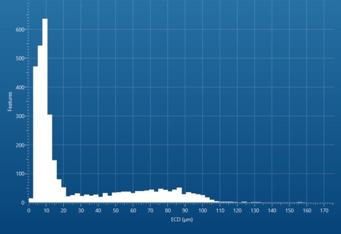
Figure 3. Histogram of the equivalent circular diameter of all powder particles detected. Image Credit: Oxford Instruments
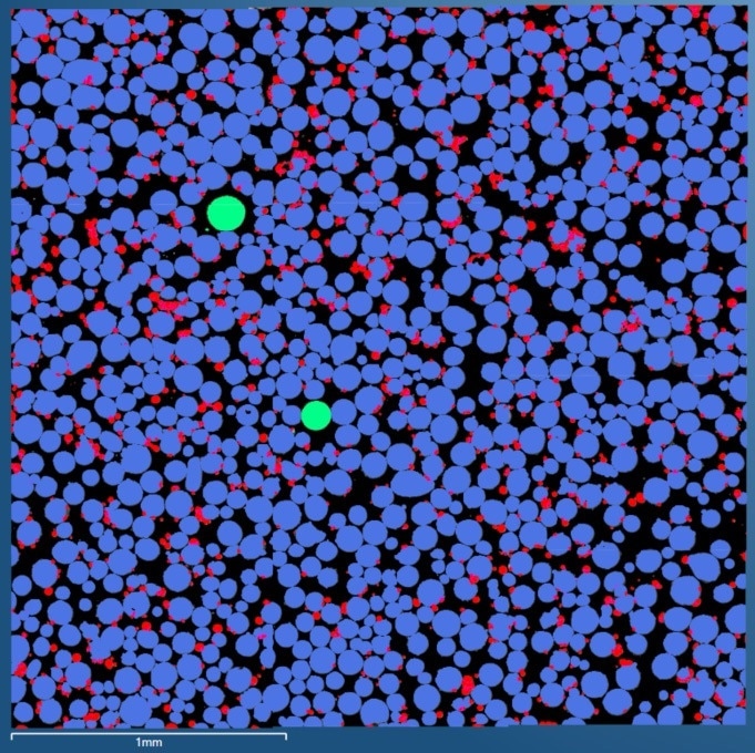
Figure 4. Particle image of complete powder sample, colour coded by class: Small Particles – Red, Large Particles – Blue and Tungsten Particles - Green. Image Credit: Oxford Instruments
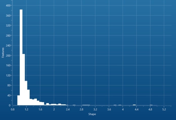
Figure 5. Histogram of shape for Large Particles in powder sample. Image Credit: Oxford Instruments
Analyzing Wear Debris
Running machines with gears and engines results in the wear of any moving components, which create wear particles in the process. Analyzing wear particles allows manufacturers to determine which components are wearing down and to predict when these components may require maintenance.
The wear particles needed for analysis can be collected by filtering them from lubricants, meaning the state of the machine can be analyzed without having to interfere with the machine itself. To carry out the analysis the wear particles were mounted on a carbon adhesive set into a TTM with the AZtecFeature.
The system can be used to analyze over an area defined by the user, or to scan over the entire sample. A disadvantage of using multiple, overlapping fields of view is some particles may appear in both images, or as fragments, and therefore be analyzed as such.
AZtecFeature automatically identifies particles which appear as fragments and digitally reconstructs them. This is highly advantageous as it means particles are not counted more than once, which would introduce error and uncertainty into the final count.
In this instance the original count gave 7,719 particles, however applying digital reconstruction reduced this number by 105 to give 7,614 particles. A categorization scheme was used to classify particles based on their major (greater than 60% by weight) elemental constitutions, with less specific particles with more unique elemental combinations placed in their own classes.
Each of these classes was assigned a color, which can be seen in Figure 6 – Mapping particles like this allows ‘problem areas’ to be identified for example, where there is too high a particle concentration for thresholding to be run. AZtecFeature can overcome these problems using advanced methods (see FeaturePhase application notes).
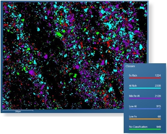
Figure 6. Wear debris particle image with particles colour coded according to class. Image Credit: Oxford Instruments
The particle categories can be used to filter the data set, meaning specific particle types can be selected for further analysis. In this example the iron-rich particles are of the most interest and the dataset is filtered for them, these particles are red in Figure 7A.
The shape of wear particles can indicate the type of wear used to produce them; for example, particles with high aspect ratios may have been produced by the stripping or cutting of their parent material. To determine if this was the case the aspect ratio of the iron-rich particles were plotted (Figure 7B). Taking approaches like this allows researchers to determine the wear mechanisms taking place.
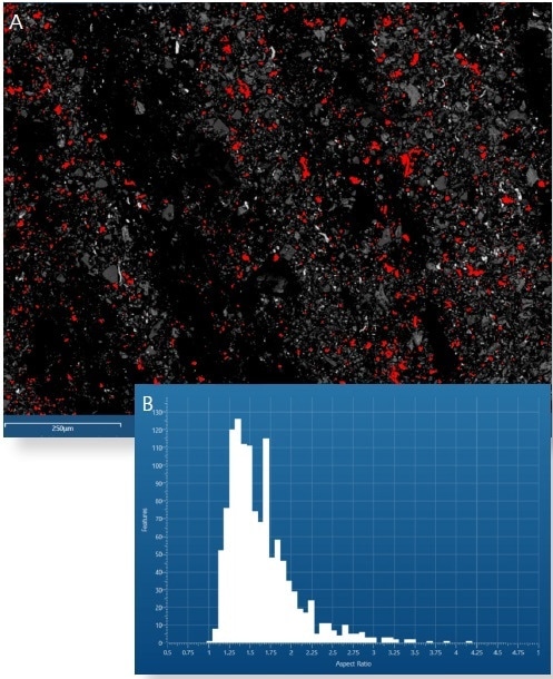
Figure 7. (A) Particle image with Fe-Rich particles coloured red. (B) Aspect ratio histogram for Fe-Rich particles. Image Credit: Oxford Instruments
In this instance the iron-rich particles tended to mostly have low aspect ratios. Monitoring if this value changes over time can be used to determine if changes in wear are occurring, and therefore if system maintenance is required.
The particle categorization used in this example was chosen using prior knowledge of the sample. However, despite this prior knowledge, 949 particles remained unclassified (colored green, Figure 6). As these particles may provide significant insight into mechanisms of wear they must also be classified. This can be achieved by simply clicking on the feature in the particle image, which provides a summary on its information (Figure 8). In this instance the particle was classified as a silicon fragment, if more silicon fragments are identified this can be set as a new category and all other relevant particles in the sample will be automatically tagged.
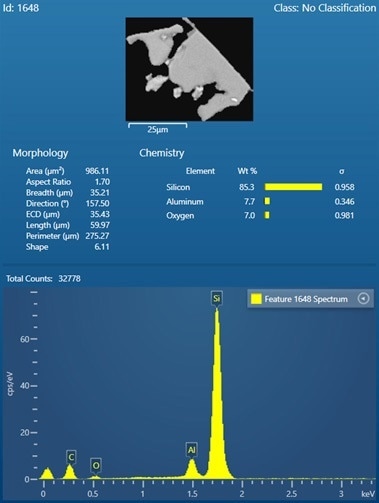
Figure 8. Summary of information for a single particle that was unclassified. Image Credit: Oxford Instruments
Conclusion
Combining a TTM with the AZtecFeature results in a versatile system for particle analysis. The system can automatically find particles in a sample and determine their shape and chemistry as a means of categorizing them. The two different examples given in this article show how the rich data provided can be used to solve analytical challenges.
The key to solving these challenges is the system’s highly flexible categorization methods and the volume of data it can use to apply these. Researchers can customize their experiments to meet the needs of their specific sample.

This information has been sourced, reviewed and adapted from materials provided by Oxford Instruments.
For more information on this source, please visit Oxford Instruments.