Spinsolve 43 MHz NMR spectrometers can be fitted with a unique sample temperature control system. This system gives users the freedom to control the temperature of the sample without needing an additional supply of nitrogen dry air or any other hardware.
This is made possible by adjusting the magnet temperature instead of using a gas flow approach, which has negative impacts on the sample volume and sensitivity of the system. The Spinsolve 43 MHz system’s variable temperature system enables customers to measure from room temperature up to 60 degrees C without compromising the resolution, sensitivity, or stability of the system.
The Spinsolve 43 MHz system includes the following features:
- A system and magnet that has been designed to allow the magnet temperature to be adjusted
- Precise temperature control for both static samples and online setups
- Compatible with standard 5 mm tubes and flow cells with no loss of sensitivity
- No need to re-calibrate the system at different temperatures
- Nitrogen or dry air supplies are not necessary
- Temperature range: RT to 60 °C
- Frequency: 43 MHz
- Available in a Standard and an Ultra version, and with added diffusion gradient
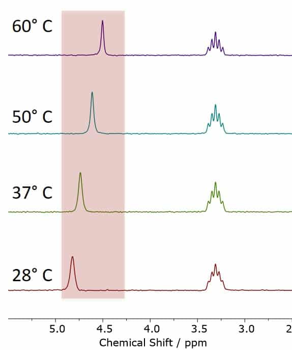
Figure 1. The MeOD-NMR Thermometer, showing MeOD spectra acquired at different temperatures between 28 °C and 60 °C. The observed chemical shift differences are in excellent agreement with the calibration values of the NMR thermometer.
Built for Stability
Using the Spinsolve multi-layer temperature control, users will not experience any reduction in the system’s stability across the entire range of temperatures.
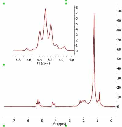
Figure 2. 100 superimposed vegetable oil spectra taken over a period of 20 hours at 60 °C. Spectra were acquired without any reshimming between measurements.
Study Reaction Kinetics
The following spectra show how easy it is to follow a rection at different temperatures. In the reaction the appearance of the ester peak and the disappearance of the alcohol peak are easy to resolve and measure. The four graphs shown in Figure 3 illustrate the concentrations acquired by integrating the ester and alcohol peaks as a function of time for a range of temperatures.
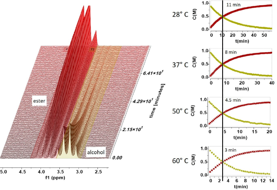
Figure 3. Concentrations acquired through peak integration.
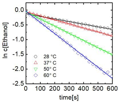
Figure 4. Plot of ethanol concentration against time.
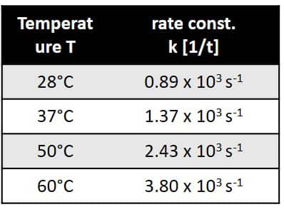
Figure 5. Temperature dependence of the rate constant.
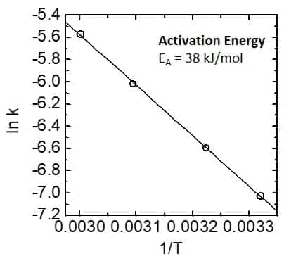
Figure 6. Activation energy graph - Arrhenius plot.
The reaction follows pseudo-first-order kinetics due to the fact that trifluoroacetic acid was used in excess.The reaction rate constants at different temperatures can be found from the slopes of the log plot. The rate constants are given in Figure 5.
By plotting the logarithm of the rate constant against T-1 and following the Arrhenius equation, it is possible to determine the activation energy of the reaction from the slope of the line. This is illustrated in Figure 6.
Improve Resolution
The linewidth in the NMR spectrum depends on two things: the homogeneity of the magnetic field and on sample properties such as viscosity. Highly viscous samples have shorter relaxation times, which result in broad lines. By increasing the temperature of the sample, the viscosity is reduced and the lines in the NMR spectrum become narrower.
Figure 7 shows the spectra of vegetable oil, recorded at 28 °C and 60 °C respectively. The improvement in the linewidth is clear at 60 °C, notice that the J-coupling splitting now becomes visible.
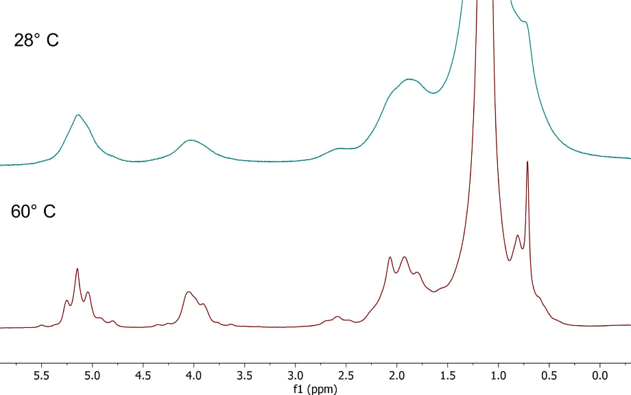
Figure 7. Spectra of vegetable oil with improving linewidth and visible J-coupling patterns.
The Spinsolve spectrometers with sample temperature control can also be equipped with pulsed-field gradients. This enables users to run temperate dependent self-diffusion studies.